 Get Started midas Civil
 Featured blog of this week

This case study covers the following aspects:
1. Introduction
2. Types of Links
3. Model Validation
4. Modeling Considerations
1.Introduction
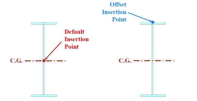
When we handle a finite element model, we might have experienced link-type boundaries. midas Civil also has link types as one of the boundary conditions. Before jumping into links, let’s look into the concept of the insertion point that can be found in a section property of midas Civil. Because the insertion point is relevant to links. When you have a beam element, it has 2 nodes at the end side. Those nodes represent the centroid of the section. Basically, the insertion point of a section is located at the centroid of the section. And the insertion point can be moved by users during modeling. We call it the offset insertion point.
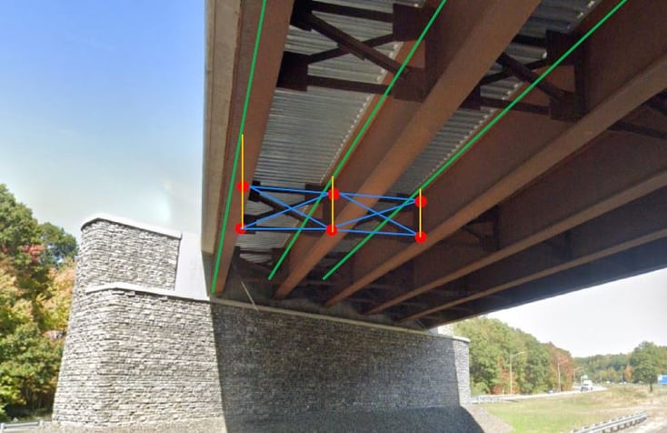
In figure 2, it shows a typical steel girder bridge. If we make up a FE model in midas Civil, green and blue lines will represent elements. Those elements have different elevations; therefore, each node of elements should be connected by links to consider the physical connections of the bridge model.
The next example, figure 4, shows a more complex bridge. This bridge has several stringers on a floorbeam, and the floorbeam is connected to truss members.
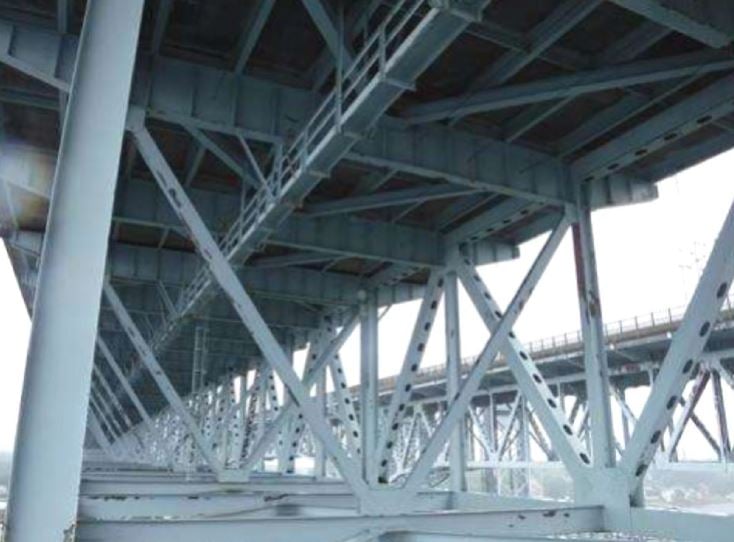
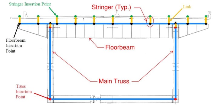
Figure 5 shows a cross-section of the bridge. Stringers, floorbeam, and main truss could be modeled as beam elements that have different insertion points. In this case, also you need to generate links on disconnected locations to consider the connection between members.
2. Types of Links
In midas Civil, there are two main types of links. One is the elastic link and the other is the rigid link. Some characteristics of elastic and rigid links are:
Elastic Links
1) Behave similar to an element.
2) User-defined stiffness to constrained DOFs.
3) Types of Elastic Links.
- Elastic – Rigid
- Elastic – Compression/Tension Only
- Elastic – General
- Elastic – Multi-linear Types of Elastic Links.
Rigid Links
1)Displacement constraint.
2)Constrained DOFs are assumed as rigid.
The elastic link behaves similar to an element in the sense that it has a stiffness in the different degrees of freedom. And it can only connect two nodes.
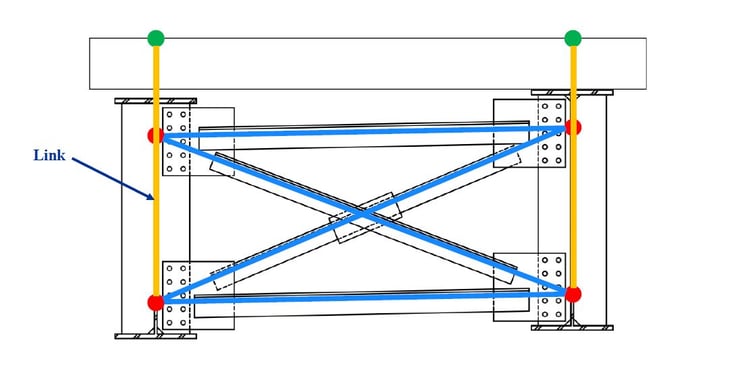
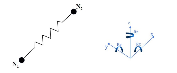 Figure 6: Concept of elements and links (Cross section view)
When you use the elastic link - rigid type, midas Civil will assign the infinite stiffness into all six degrees of freedom. The stiffness is relatively higher than the elements surrounding. This type can be used for supports and diaphragms.
The other type of elastic link is the elastic link – compression/tension type. This type has only an axial stiffness. It can be used for special configurations and a model having the soil-structure interface such as an integral abutment. Especially, you should know that this type is a non-linear link. The next one is the elastic link – general type. This type can give you the most flexibility in the definition of stiffness. You can define stiffness in all six degrees of freedom manually. This type is typically used in areas where only some DOFs need to be constrained and stiffness in other DOFs is known.
Let’s move onto the rigid link. The rigid link is similar to the geometric constraint. This type can be linked to more than two nodes. When you define a rigid link, you need to define a master node and a slave node. The distance between the master node and the slave node will be constant during analysis. It means if the master node is translated or rotated, the slave node will have the same behavior with the constant distance.
Typical applications are:
-
At beam elements to plate elements transitions.
-
At girder ends/supports.
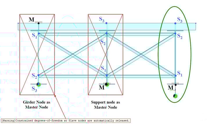
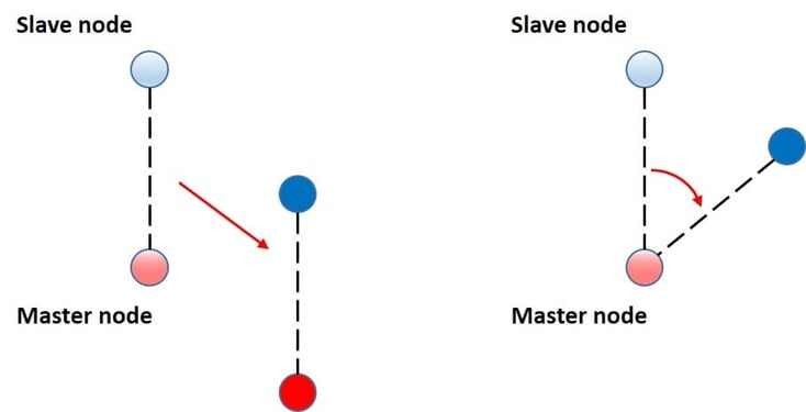
Figure 9: Application of rigid links at girder ends/supports
The most typical application of rigid links might be found at the ends of girders for support conditions. Figure 9 shows three different configurations of rigid links. The first example is ‘Girder Node as Master Node’. In this case, the master node doesn’t have a support condition. On the other hand, the slave node has a support condition. The characteristic of the rigid link is that slave nodes are constrained at a master node. Therefore, the support condition on the slave node will be ignored during analysis and you can see the warning message shown in figure 9. The second case is similar to the first case. It has a master node at the bottom. A support condition is assigned to the master node. This case is a bit tricky to catch something wrong because this model is stable. In this case, several slave nodes connected to a master node therefore, the support conditions on the master node will be applied to those slave nodes. It possibly can make wrong results. The correct configuration is to have an additional node at the bottom of the girder node and to add an elastic link between nodes.
3. Model Validation
Model validation is critical for the proper use of links and boundary conditions. One of the approaches for applying links is to build a model with all links DOF constrained and to validate structure behavior. After that, release DOFs gradually to ensure there are no instability issues and to validate structure behavior along the way. Typical items to validate are bending moments, deflections, and intended load path.
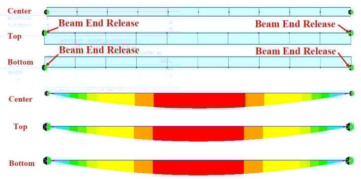
Here is the first validation example. Figure 10 shows a simply supported beam. This example shows that incorrect results can occur even links properly defined. Figure 10 shows the negative moments at the end of the beam. This result obviously isn’t that correct. In order to make it the correct way, you should use Beam End Release function at the end of the beam element.
/Contents/Tips%20Tutorials/new%20image%20Application%20of%20Links%20in%20Bridge%20FE%20Models/Bending%20moment%20result%20of%20simply%20supported%20beam.png?width=734&name=Bending%20moment%20result%20of%20simply%20supported%20beam.png)
Figure 10: Bending moment result of simply supported beam
/Contents/Tips%20Tutorials/new%20image%20Application%20of%20Links%20in%20Bridge%20FE%20Models/Bending%20moment%20result%20of%20simply%20supported%20beam%20with%20Beam%20End%20Release.png?width=734&name=Bending%20moment%20result%20of%20simply%20supported%20beam%20with%20Beam%20End%20Release.png)
Figure 11: Bending moment result of simply supported beam with Beam End Release
The second example is regarding the insertion point and offset insertion point. If you assign an offset insertion point, midas Civil will internally create the rigid link between an original point and offset insertion point. It makes the same issue as the first example as shown figure 12 and 13.
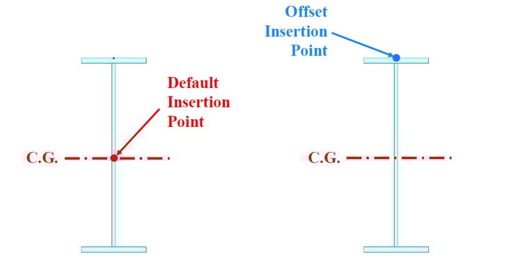
Figure 12: Insertion point and offset insertion point
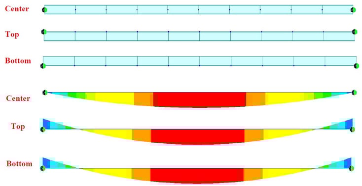
Figure 13: Results along the insertion point
The third example is a truss bridge. After analysis, the results seemed to be fine however, member force results have shown huge bending moments at the ends of the bottom chord. This model has diagonal members. Especially, diagonal members at the end of the truss had the offset insertion point. It made improper results. After the change of insertion point, analysis results showed reasonable values. It is a good example that shows a small input could hugely influence analysis results.
/Contents/Tips%20Tutorials/new%20image%20Application%20of%20Links%20in%20Bridge%20FE%20Models/Initial%20bending%20moment%20results%20with%20offset%20insertion%20points.png?width=734&name=Initial%20bending%20moment%20results%20with%20offset%20insertion%20points.png)
Figure 15: Initial bending moment results with offset insertion points
/Contents/Tips%20Tutorials/new%20image%20Application%20of%20Links%20in%20Bridge%20FE%20Models/Modified%20bending%20moment%20results%20with%20original%20insertion%20points.png?width=734&name=Modified%20bending%20moment%20results%20with%20original%20insertion%20points.png)
Figure 16 : Modified bending moment results with original insertion points
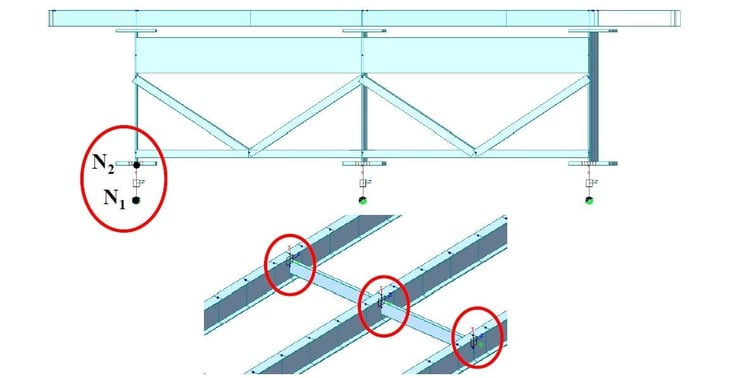
The fourth example is a connection between a stringer and a floorbeam in the same truss bridge. The stringers are supported on the floorbeams. Several rigid links are used for this case. The stringers are continuous on the floorbeams. Therefore, the initial expectation was that positive bending moments occur between floorbeams and not big negative moments occur at the floorbeam locations. However, analysis results showed that not making sense.
/Contents/Tips%20Tutorials/new%20image%20Application%20of%20Links%20in%20Bridge%20FE%20Models/Rigid%20link%20details.png?width=734&height=491&name=Rigid%20link%20details.png)
Figure 17 : Rigid link details
/Contents/Tips%20Tutorials/new%20image%20Application%20of%20Links%20in%20Bridge%20FE%20Models/6.png?width=734&name=6.png)
Figure 18 : Initial bending moment results
The reason for this issue was that the rotation of the master node introduces additional moments on the stringers. So, the moment in the y-axis was released using Beam End Release. After that, this issue easily was figured out.
/Contents/Tips%20Tutorials/new%20image%20Application%20of%20Links%20in%20Bridge%20FE%20Models/Initial%20bending%20moment%20results.png?width=734&name=Initial%20bending%20moment%20results.png)
Figure 19: Modified bending moment results with Beam End Release
The last example is a bridge having high skew. This bridge has two main girders along the traffic direction. And it has several diagonal members between two girders and a diagonal joint at the middle of the bridge.
/Contents/Tips%20Tutorials/new%20image%20Application%20of%20Links%20in%20Bridge%20FE%20Models/Bridge%20overview.png?width=734&name=Bridge%20overview.png)
In terms of the diagonal joint, it was designed as fixed at the left side and movable at the right side of the deck. An initial issue was that the movable side could introduce damage to the deck along the time. Therefore, a new bearing system was proposed. It was a tie-down system. This type can prevent the damage of the deck and allow it to expand itself. For the design, there were steps the engineer needs to check. The first one is what causes a hammering effect on the deck. And the second one is to find a design load.
/Contents/Tips%20Tutorials/new%20image%20Application%20of%20Links%20in%20Bridge%20FE%20Models/Bearing%20overview%20(Existing%20vs%20Proposed).png?width=734&name=Bearing%20overview%20(Existing%20vs%20Proposed).png)
There were two main configurations that have been found. When truckloads are placed on the south and north side of the joint, it causes a vertical gap on the joint. And when truckloads are placed on one side of the joint, it also causes a vertical gap on the joint. In order to model the bridge in midas Civil, elastic links have been used.
/Contents/Tips%20Tutorials/new%20image%20Application%20of%20Links%20in%20Bridge%20FE%20Models/Vertical%20gap%20at%20the%20join%20(Case%201).png?width=729&name=Vertical%20gap%20at%20the%20join%20(Case%201).png)
/Contents/Tips%20Tutorials/new%20image%20Application%20of%20Links%20in%20Bridge%20FE%20Models/Vertical%20gap%20at%20the%20join%20(Case%202).png?width=729&name=Vertical%20gap%20at%20the%20join%20(Case%202).png)
/Contents/Tips%20Tutorials/new%20image%20Application%20of%20Links%20in%20Bridge%20FE%20Models/12.png?width=731&name=12.png)
4. Modeling Consideration
The last part is how to consider what type of links you should use. The first step is to check out what degrees of freedom need to be constrained. You can choose a suitable one among link types depending on degrees of freedom. The second step is to consider the size of the model and computation time. This is not big deal on a small model but if the model is getting bigger, proper link types can influence the model and analysis. The third step is to consider whether you need member forces at a link location or not. If you need the member forces, the elastic link will be a suitable case. The last step is to validate your model even the model is simple and small. It will be helpful to improve the quality of your model.
Watch the full webinar video