 Get Started midas Civil
 Featured blog of this week

Watch the full webinar video
Please fill out the Download Section (Click here) below the Comment Section
to download the Full Webinar Presentation File.
*Click the content to move to the section
This case study covers the following aspects:
1. Project Information
2. Review of Modelling Details in midas Civil
3. Design and Checking Results
1. Project Information
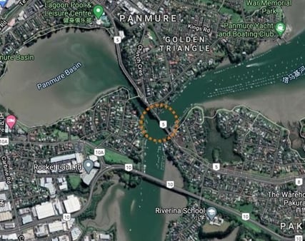
The Panmure Busway bridge is located in Panmure, Auckland, New Zealand. The bridge is across the Tamaki River and is part of the Auckland Eastern Busway project. The client was Auckland Transport and the designer for this bridge was Beca Ltd. The design features include the provision of 3.3m bus lanes and a 4.97m footpath and cycleway incorporating a viewing platform at each abutment and pier on the northern end of the proposed busway bridge. The scope of the project includes eastern and western abutment retaining, approach embankment, batter slopes, and a sheared path connecting the Rotary Walkway on the northern side of the Pakuranga Road.
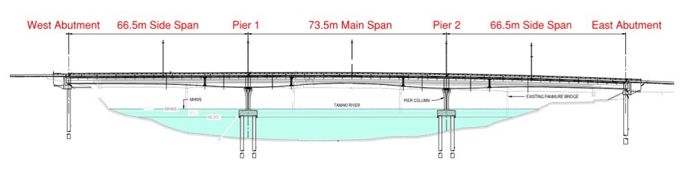
The bridge is a three-span steel composite I-girder bridge with a total length of 206.5m. The main span is 73.5m long and the side spans are 66.5m long. This bridge is supported by abutments at both ends and two large piers with 8 piles each between spans. The superstructure is comprised of two parallel composite steel I-girders supporting the road carriageway, footpath, and cycleway with no vertical structure above deck level. The girders are launched, varying in depth from approximately 3.8m over river piers to approximately 2.3m at each mid-span both for economy and shape for architectural reasons. Steel cross girders are provided between the main girders.
The girders are continuous over the piers. Bracing between girders is provided 10.5m from the piers to limit the buckling length of compression flanges. The deck slab consists of 125mm thick precast concrete deck panels spanning between the cross girders, with a 125mm thick cast-in-situ concrete topping.
/Three-Span%20Steel%20Composite%20I-Girder%20Bridge%20Design/How%20I%20Designed%20a%203-Span%20Steel%20Composite%20I-Girder%20Bridge/Plan%20View%20of%20Bridge.png?width=728&name=Plan%20View%20of%20Bridge.png)
/Three-Span%20Steel%20Composite%20I-Girder%20Bridge%20Design/How%20I%20Designed%20a%203-Span%20Steel%20Composite%20I-Girder%20Bridge/Cross-Section%20View%20of%20the%20Superstructure.png?width=734&name=Cross-Section%20View%20of%20the%20Superstructure.png)
2. Review of Modeling Details in midas Civil
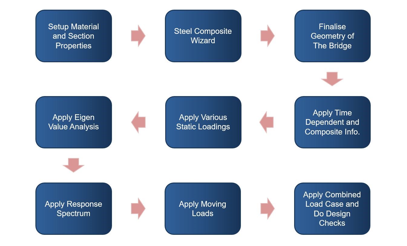 Figure 5: Workflow
Let’s take a look at the overall workflow while building the global model together using midas Civil. The process is as follows:
a) Setup the materials and section properties.
b) Use the Steel Composite Wizard function to set up the main superstructure of the bridge. It offers some very handy options for setting up the model.
c) Generate additional elements after using the wizard function.
d) Apply the various loadings, time-dependent material for construction staging, and conduct eigenvalue analysis for seismic loading.
e) Apply the moving loads to stimulate the forces that the bridge experiences from vehicles. It is worth running the model a couple of times when building it to make sure that the model behaves as expected.
f) Create the load combinations using the New Zealand Bridge manual or national design code to complete the model for design checks.
2-1. Review of Steel Composite Bridge Wizard
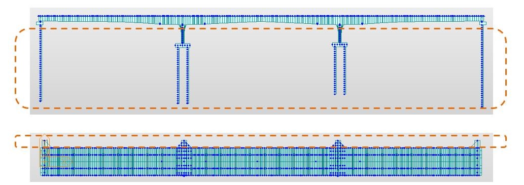
Steel Composite Bridge Wizard starts with the basic geometry of the bridge. Firstly, the user will see the ‘Layout’ tab when using the wizard. Here, we can choose a modeling method for a superstructure and also whether to include elements for a substructure or not. For this bridge, the general geometry is set up with the piers to simplify the process of building the rest of the substructures such as pile caps and piles. The input parameters can be obtained from concept design drawings. The elastic link stiffness defines the boundary condition between the piers and the superstructure. One tip for using the wizard function is to identify and input all the materials and section properties in midas Civil before using the wizard function to set up the geometry, loading, and staging faster.
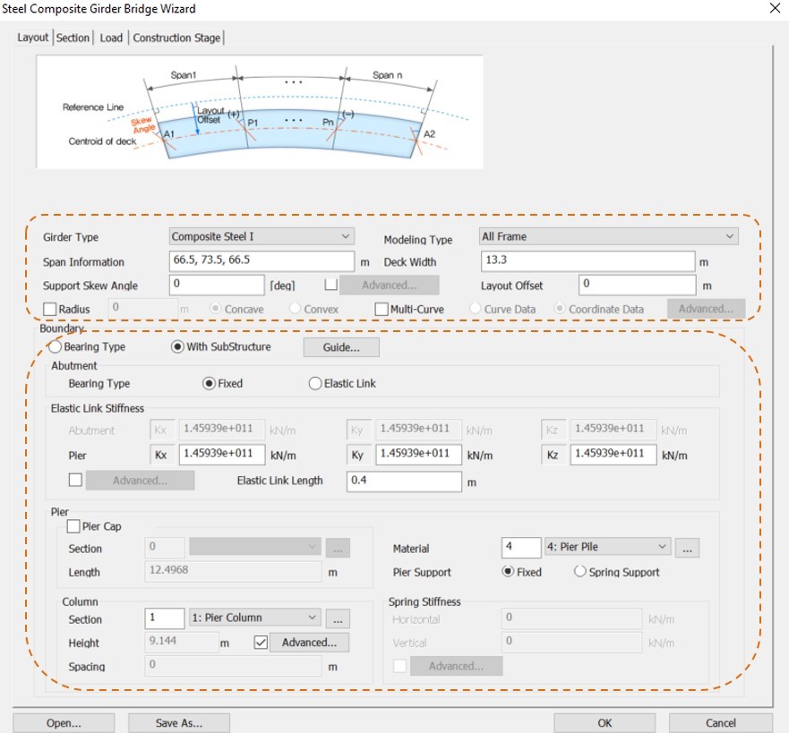
The bridge is designed with two main I-girder beams running across the bridge. It is symmetrical from the middle of the bridge. Therefore, the superstructure can be easily generated by selecting a grillage model called ‘All Frame’ in the layout tab.
/Three-Span%20Steel%20Composite%20I-Girder%20Bridge%20Design/How%20I%20Designed%20a%203-Span%20Steel%20Composite%20I-Girder%20Bridge/Typical%20Cross-Section%20View%20of%20the%20Bridge.png?width=734&height=697&name=Typical%20Cross-Section%20View%20of%20the%20Bridge.png)
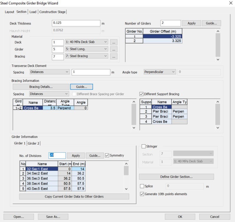
Next to the layout tab, we can see the ‘Section’ tab. Here, the user can allocate the materials and section properties of the deck, girder, and bracing along with the deck thickness. Furthermore, the user can input detailed superstructure shapes such as the number of girders and the position of girders. A useful tool is the ‘copy current girder data to other girders’ tab where the user can duplicate the position data from one girder to all the other girders. This saves the user time from manually inputting the data.
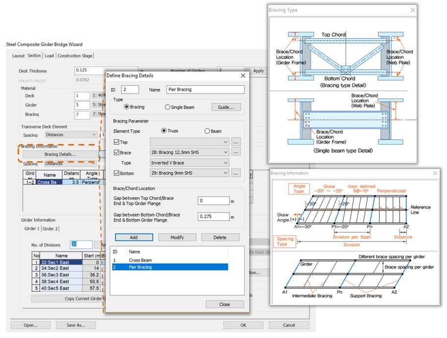
In the bracing details option, the user can select different bracing types and details. For this bridge, there are two types of bracing, the cross beam and the bracing at the pier as shown in figure 7. This option allows the user to set up various types of bracing which saves the user time from manually drawing the model. Furthermore, it automatically generates the boundary conditions and geometry of the bracing, speeding the modeling process.
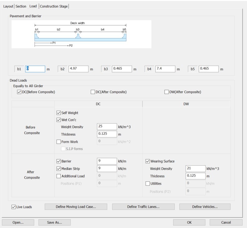
Let’s move onto the ‘Load’ tab. Over here, the user can input typical design forces which will save the user time afterward. This option allows the user to add loads such as self-weight, the weight of wet concrete, and the barrier. These dead loads can be applied to each construction phase automatically if the construction stage analysis is considered. Because the model is a highway bridge, moving loads such as traffic loads were also considered (Users can input the information about the moving load such as traffic lane and vehicles as well.) This can save the user time assigning them later on in the process.
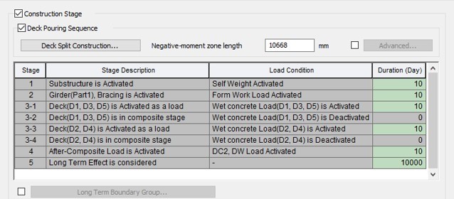
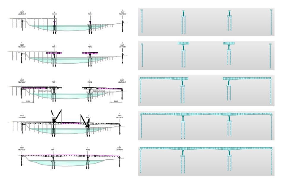
The last part of the wizard is the ‘Construction Stage’ tab. The construction staging for the bridge consists of 10 steps with two stages of deck pour sequence. The wizard allows users to specify negative moment zone length which correlates to the mid girder span length shown at stage 4. The construction staging of the bridge has been carried out by this tab. The construction stage tab provides the ‘Deck Split Construction’ option to define detailed steps in the same stage. This allows users to capture all design scenarios through the full construction of the bridge.
If the user needs to create construction staging for the model from scratch, then a good practice is to ensure the user to have the correct structure groups, boundary groups, and load groups when setting up the model.
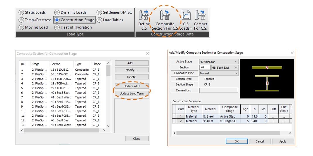
One of the key parts for setting up the construction stage is the composite section for C.S. It is important to make sure that all component types are either composite or tapered composite when setting up the material and section properties. In this function, users can activate a part of a section individually with information about the material and the age of the part. The H value and long terms are automatically generated, so the user can input a calculated arbitrary value and then check updates and all H values. Thereafter, update the Long term once the user completes the setup. It is critical that the user finishes this step correctly as it can significantly affect the analysis result.
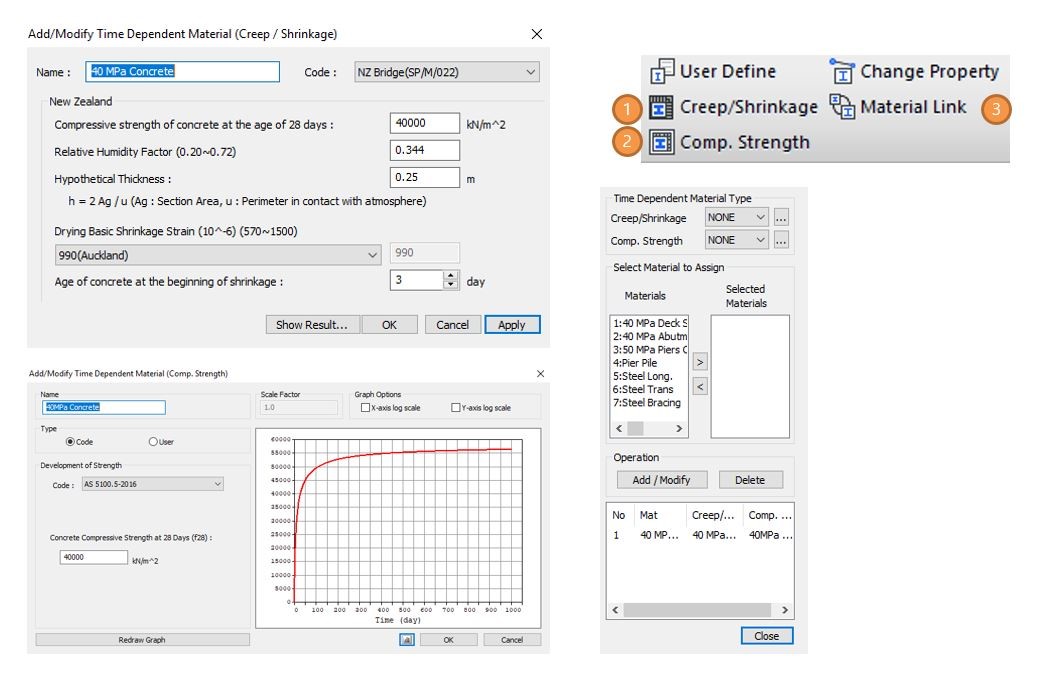
The time-dependent material is a useful function to capture the creep and shrinkage loadings. The creep and shrinkage function allows the user to input parameters from the Bridge Manual. There are changes in the latest edition of the New Zealand Bridge Manual on the drying basic shrinkage strain which can be easily adjusted by selecting the user-defined options. These creep and shrinkage loadings are captured after the user applies the construction staging loadings
The Steel Composite Bridge Wizard is a great tool to help the designer build the superstructure of the bridge as well as applying some basic loading and construction staging for the model. However, it comes with some limitations. For the bridge in this project, there were some works required after using the wizard to complete the modeling.
The first part is building the substructure of the bridge. While the wizard provided a great starting point for building the substructure, the pier cap, pier, pile cap, and piles need modeling in the actual modeling interface. Since the bridge has four deck extensions on each side, the geometrical shape is not typical. Therefore, the deck extensions need to be modeled separately. Those components were built after the wizard.
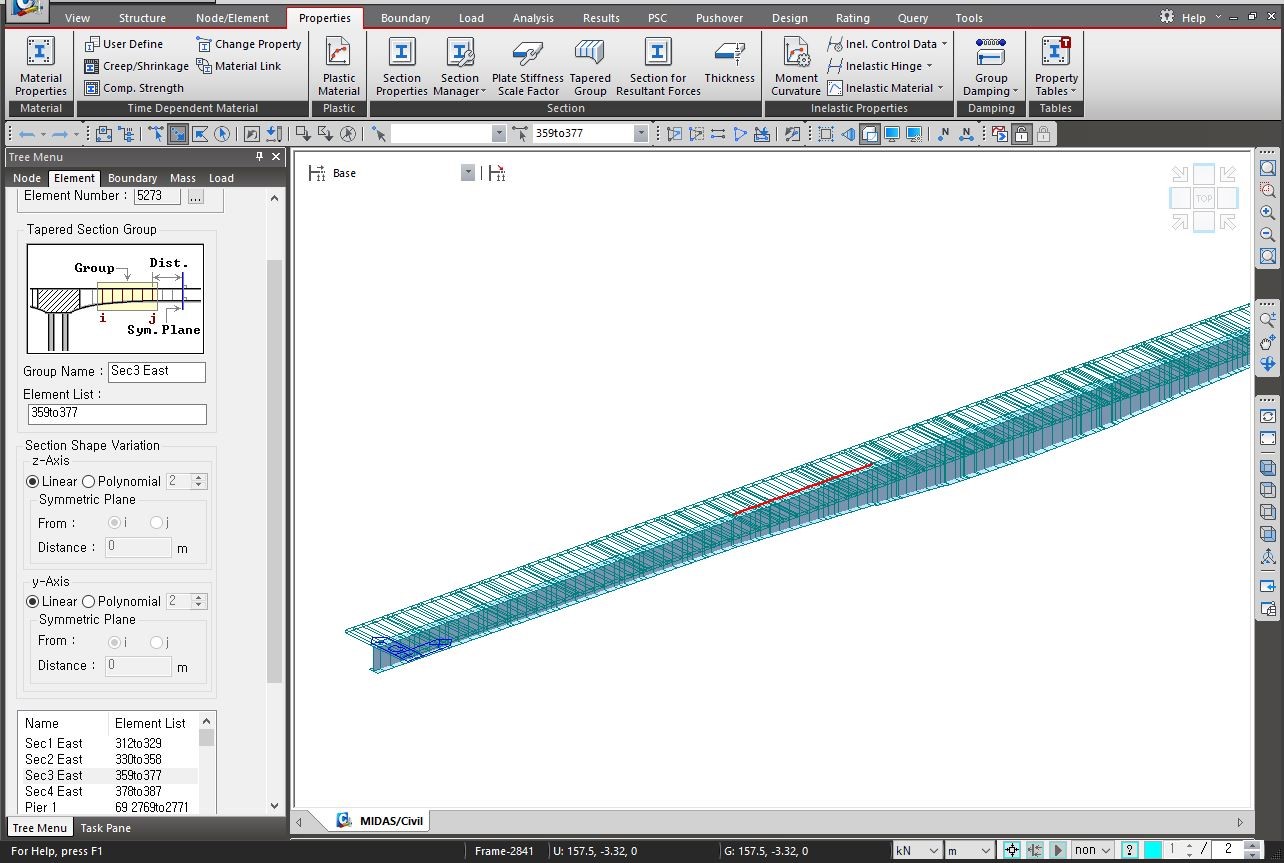
The second part is to apply the tapered section groups for the superstructure and substructure of the bridge. Due to the unique geometry of the bridge, the tapered section groups were applied to the steel girders and piers to finalize the geometry shape of the bridge for the modeling.
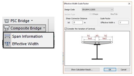
The third part is to apply the composite information such as effective width scale factor and composite span information. This can be found under the structure tab composite bridge. The effective width of the bridge is modeled in midas Civil to capture the effect of shear lag. This is compared with manual calculation from AS5100.6 to ensure that the model inputs are equivalent to the Australian Standard. Our comparison found that the effective width calculated from the model was very similar to the effective width found from AS5100.6, and this was used for the analysis.
2-2. Review of Boundary Condition
The boundary condition for this steel composite bridge is quite standard. The bearing design philosophy is as follows:-
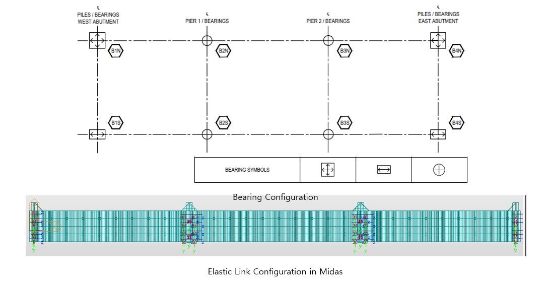
At the piers, all the bearings are assumed to carry an equal portion of longitudinal and transverse loading. At each abutment, the guided bearing is assumed to carry all the Ultimate Limit State (ULS) static or serviceability limit state (SLS) 3A case in the bridge manual for transverse loading. The guided bearing on either end of the bridge is allowed to fail under large seismic events, which in this case the concrete shear key will be engaged to provide transverse restraint. The bearing restraint in the bridge was modeled using the Elastic Link in midas Civil. The elastic link is a good boundary condition function that allows the user to find the resultant loads easily through the result tables.
To apply soil springs to the piles, a particular workflow was used to speed up the process. After constructing the geometric model in midas Civil, use the ‘renumber element ID’ under the structures tab to renumber pile node ID in ascending orders. Then move onto the ‘Point Spring’ function to apply the soil spring. Then input an arbitrary number such as 1 to the stiffness of the spring for all pile springs so a table is produced. If the construction stage is planned, please make sure to define the boundary group for all the pile soil springs. This will easily add boundary groups to the construction staging.
In the point spring table, order the pile in ascending order by the node ID. This way, the soil spring value could be copied and pasted from an excel spreadsheet that contains all the soil spring values, provided by Geotech engineers, to the point spring supports the table. This makes the application of soil spring value much easier, particularly for structures that contain a lot of piles.
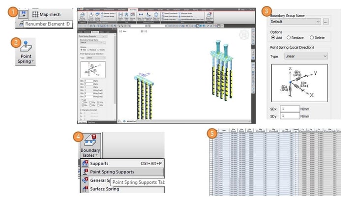 Figure 19: Workflow for soil parameter
2-3. Traffic Loading
The traffic loadings in New Zealand Bridge Manual consist of normal vehicle loads and overload vehicle loads as shown in figure 20. The application for the loading is quite straight forward with a 120kN axle load spaced 5m apart and a UDL of 10.5kN/m for normal vehicle load and a 240kN axle at 5m apart with UDL of 10.5 kN/m for the overload vehicle load. There is a reduction factor dependent on the number of loaded lanes and the dynamic load factor dependent on the type of structure and clear span length.
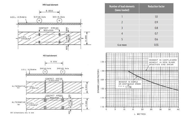
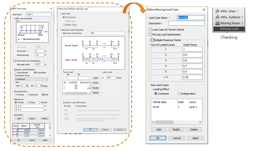
Figure 21 shows the application of traffic loadings in midas Civil. Since the reduction factor between the Canada Code and the NZ Bridge Manual are the same, the Canada code for moving load application was selected. When a traffic lane was defined, the ‘Transverse Lane Optimization’ option was checked to conservatively analyze the bridge subjected to moving load. In order to cover all case scenarios, the application of vehicle loads was considered, and also moving loads for pedestrian cycling were also considered to simulate the worse scenarios.
‘Define Moving Load Case’ function allows users to set up the different loading scenarios with different vehicles on different lanes. When checking the result for the moving load cases, users can use the moving tracer to see which vehicles and load cases were causing the critical moment/shear demand on the bridge. This will give users a bit more confidence that the moving load case makes sense with the predicted scenarios.
2-4. Temperature Loading
The temperature effect has also been taken into consideration for this bridge structure. Section 3.4.6 in the NZ Bridge Manual outlines the load application for both uniform temperature change and differential temperature change. In midas Civil, ‘Element Temperature’ load type was applied to consider the temperature difference.
For differential temperature, the ‘Beam Section Temperature’ load type was selected. The temperature gradient was calculated using an excel sheet with Bridge Manual code and AS5100.2 for a negative temperature gradient. Then, the temperature load was applied along the full depth of the steel composite girder.
/Three-Span%20Steel%20Composite%20I-Girder%20Bridge%20Design/How%20I%20Designed%20a%203-Span%20Steel%20Composite%20I-Girder%20Bridge/7.png?width=734&name=7.png)
2-5. Water Flow Loading
Since this bridge is spanning over a river stream, a unique load case should be considered. That is the water flow loading. This is a load case that captures the water flow load through the piers in both the transverse and longitudinal directions. AS5100.2 section 16 was used to determine the design drag force that was applied in midas Civil. The force was applied in both longitudinal and transverse directions to cover the critical case scenarios. These were translated into ‘Line Beam’ load types on the piles and piers. After the analysis of the bridge, it was found that the water loads were insignificant when compared to seismic and wind load, so it did not govern the bridge design.
/Three-Span%20Steel%20Composite%20I-Girder%20Bridge%20Design/How%20I%20Designed%20a%203-Span%20Steel%20Composite%20I-Girder%20Bridge/Water%20flow%20load.png?width=734&name=Water%20flow%20load.png)
2-6. Response Spectrum
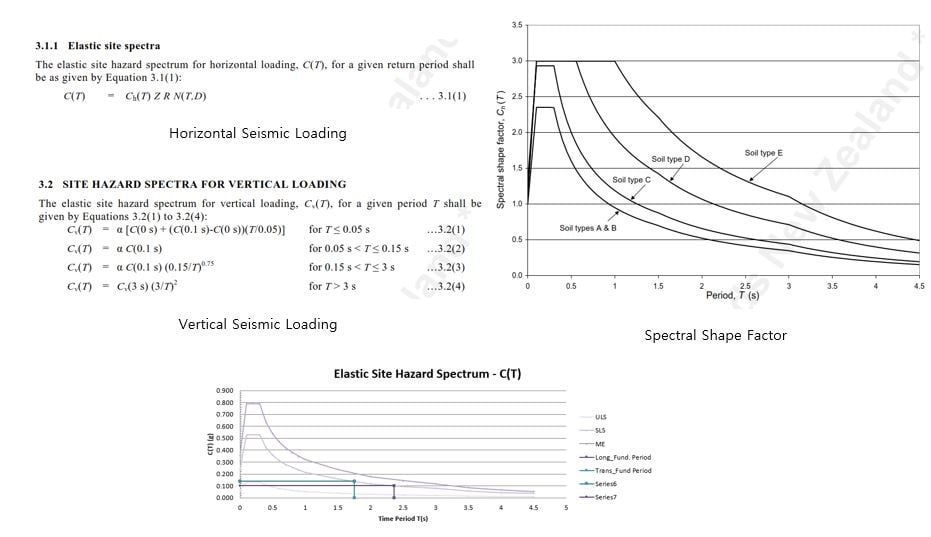
There are two types of seismic loadings that are considered for seismic, horizontal, and vertical seismic loads. The horizontal and vertical seismic loads dependent on the spectral shape factor, hazard factor, which is based on the region, the return period factor, and the near-fault factor. The application of horizontal seismic load is dependent on the natural period of the structure that is obtained through the eigenvalue analysis. Figure 24 shows the elastic site spectra formula in the NZS 1170.5 standard for both horizontal and vertical seismic loads as well as the spectral shape factor.
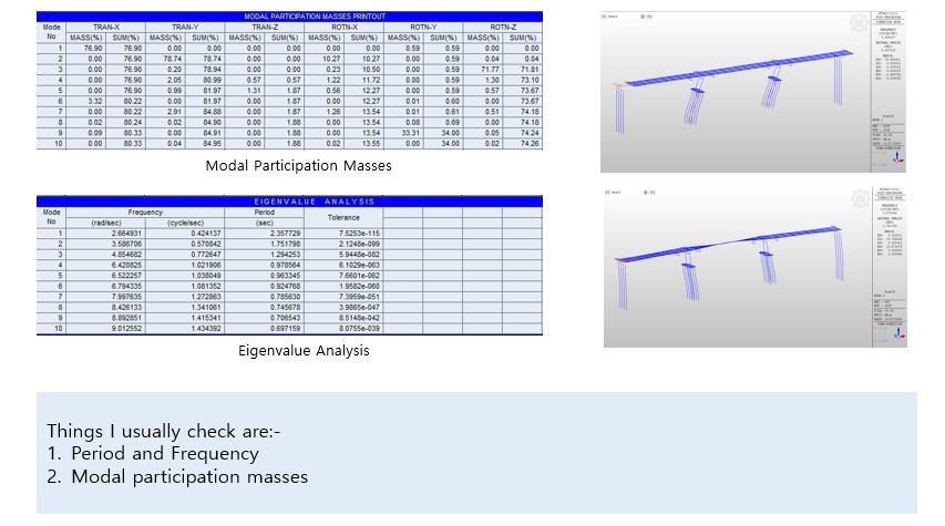
In order to add seismic loads to the analysis, the first thing to do is to perform an eigenvalue analysis. Depending on the structures, users can adjust the number of frequencies in the analysis in order to get a higher mass participation ratio. After finding the natural period of the structure through eigenvalue analysis, define the response spectrum function that can be inputted using the ‘RS Function’ in midas Civil. Then, move onto the ‘RS Load Cases’ function to create load cases. This allows users to specify the direction of the seismic excitation. The scale factor is determined through iterations of calculating the equivalent static-based shear force result analysis and the response spectrum analysis. The modal combination control is where users can choose to add direction signs to the result as well as choose between different seismic analysis methods.
Note: There are two options for adding signs to the results,
- Add along the major mode direction.
- Add along the absolute maximum value.
If the second option is selected, it can be the maximum value in different directions which can cause an abnormal deformation in the model, whereas selecting along the major mode application direction will give the user a real deformed shape under seismic loading.
/Three-Span%20Steel%20Composite%20I-Girder%20Bridge%20Design/How%20I%20Designed%20a%203-Span%20Steel%20Composite%20I-Girder%20Bridge/Quick%20review%20on%20how%20to%20apply%20the%20response%20spectrum%20in%20midas%20Civil%20%C2%A0.png?width=734&name=Quick%20review%20on%20how%20to%20apply%20the%20response%20spectrum%20in%20midas%20Civil%20%C2%A0.png)
To find the natural period for the structure, it is important to check the modal participation mass to see what percentage of mass is contributed under a particular mode. In this case, the first mode is the longitudinal seismic case and mode 2 is the transverse seismic case. The user can also identify this by looking at the deformation shape of the structure. This can be accessed by clicking on the mode shape button in midas Civil. After the right natural frequency is found, the user can use the NZS1170.5 or the national design code to calculate the response spectrum profile and apply it in midas Civil. With some iteration of seismic load comparison between outputs from response spectrum and equivalent static base shear, the user can find the right scale factor to apply to the longitudinal and transverse seismic cases. This completes the seismic analysis part.
3. Design and Checking Results
AS5100.6 was used for the design checks, with the help of Midas Civil. For the main bridge, the NZTA RR Bridge Manual, and for the splices, the British Standard. Basically, data was extracted from the result tables in midas Civil. Thereafter, a spreadsheet was used to conduct design checks for the bridge. From the wizard, moving load analysis and response spectrum were able to complete the design checks for the bridge within the allowed time frame, which proved the efficiency of midas Civil for design.
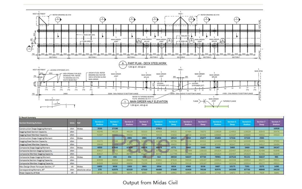
A good practice is to understand the midas result table data so users can extract it from excel and process it to find the required one. It is a good practice to use the result table to extract the loading rather than the model itself because the value the user gets is more accurate. The result display in the model is good for understanding the behavior of the structure and where the critical loads are located; whereas the result table gives accurate demand values.
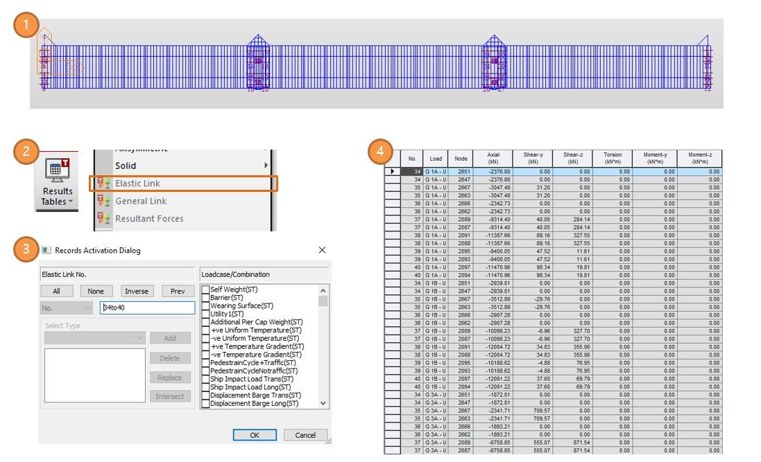
Figure 28: Bearing check in midas Civil
The bearing design can be checked directly from the model. To check this, the user must first identify the elastic link ID that represents those bearings. Then goes to the ‘Elastic Link’ under the results table to activate the result table for the bearings. The data in the spreadsheet shows the loads that the elastic link or bearing is transferring from the superstructure down to the substructure via different load cases. The user can sort the load directly from the table or export it to excel for data processing in order to find the critical load for bearing design.
Q&A
Question 1
How do you design the shear keys considering the longitudinal shear?
Answer 1
Longitudinal shear reactions for the shear studs were obtained from Midas Civil at the joint locations. We output the vertical shear force from Midas Civil and then check the design using section 4.8 of AS5100.6
Question 2
How do you model the pier headstock?
Answer 2
The pier headstock sections were drawn in AutoCAD and imported as a tapered general section.
Question 3
How do you consider the shear lag effect in your model?
Answer 3
We used the Effective Width Scale Factor function under the composite bridge in the structure tab to capture the shear lag effect.
Question 4
Can you please explain transverse load optimization during traffic loading?
Answer 4
In midas Civil, the traffic loading is placed in the middle of the influence line/surface. If Transverse Lane Optimization is checked on, the traffic loading will be applied for cases for the right/left end of a lane.
Question 5
Re: transverse load optimization, if the traffic lane is 3.5 m wide should we limit the optimization width to 3.5 or we should go beyond this value if the bridge deck is wider?
Answer 5
It is limited in the total width of a lane.
Question 6
How do you determine the crack zone length of the concrete deck over the internal support? And what is the 1st frequency of this bridge?
Answer 6
A separate plate model has been built to check the concrete deck, full crack property at the hogging moment zone might be assumed for the design. The first frequency of this bridge is 0.424 cycles/sec.
Question 7
Is the deck cast on-site or precast, is there any difference in modeling in midas Civil?
Answer 7
The deck is made of a 125mm precast and a 125mm cast in situ slabs. It is modeled as a single 250mm thick concrete slab.
Question 8
How do you design the shear keys considering the longitudinal shear?
Answer 8
Longitudinal shear reactions for the shear studs were obtained from Midas Civil at the joint locations. We output the vertical shear force from Midas Civil and then check the design using section 4.8 of AS5100.6