Structural Connections and Contacts

Structural Connections and Contacts

Table of Contents

1. Importance of Modeling Structural Connections

2. Modeling Structural Connections in Finite Element Analysis

3. Types of Structural Connections and Joints

4. Types of Contact in FEA

5. How does FEA Software Simulate Contact?

6. Examples of Contact Modeled in Finite Element Analysis

1. Importance of Modeling Structural Connections

Structural connections are usually the weakest part of a steel structure; however, they are rarely the subject of structural analysis. To simplify the analysis, engineers use elastic links with reduced elastic modulus to simulate structural connectors’ effect on the general structure. However, the structural connectors themselves may experience failure due to the general structural behavior, and their nonlinear complexities may not be approximated by an elastic link. A connection may involve complicated geometry, misalignment, different materials, prestress, making or breaking of contacts, friction and slippage, plastic action, and damage to the material from bending, welding, and punching holes [1].

2. Modeling Structural Connections in Finite Element Analysis

Due to the complexities in geometry and structural behavior, detailed FE analysis is needed for structural connectors. Detailed analysis requires engineers to produce a realistic CAD, which can be built in CAD software and then exported to FEM software. The CAD models can also be directly built in FEM software to mesh and perform finite element analysis (watch how to create irregular geometry and mesh in a detailed analysis software here). Figure 1 shows the I girder splice connection modeled as plates and meshed using plate elements in Midas FEA NX. Figure 2 shows the solid model and mesh of the same structural connection. To read more on the pros and cons of using plate (2D) and solid (3D) elements for FEA, go to Basic Finite Element Mesh Explained.

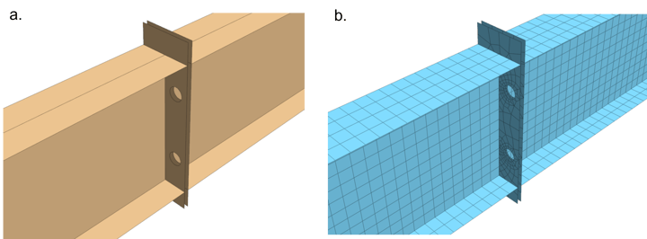Figure 1. (a) Plate model of the splice girder connection created in midas FEA NX. (b) Plate mesh of the splice girder connection created in midas FEA NX.

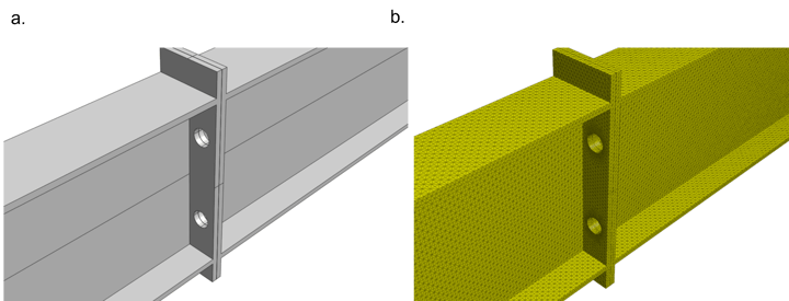
3. Types of Structural Connections and Joints

Some common structural connections seen in steel bridges are beam-to-beam connection, beam-to-column connection, flexible end plate connection, fin plate connection, splice connection, bolted column bases, etc. The listed connections all involve having multiple structural components coming into contact and utilizing friction and can be simulated using contact analysis in finite element tool Midas FEA NX.

4. Types of Contact in FEA

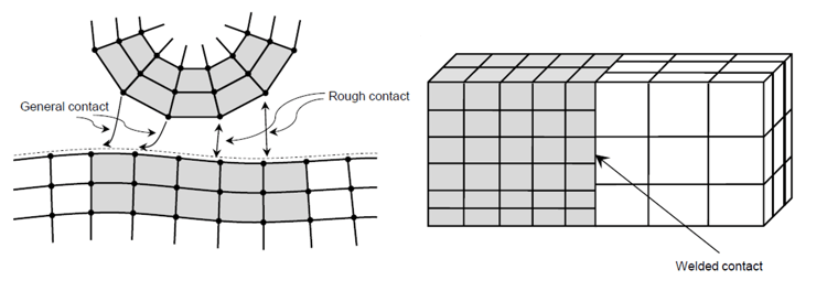
Contact analysis fundamentally assumes that two objects in a space can be in contact, but cannot penetrate each other (non-penetration condition), and are nonlinear in behavior. The common types of contacts are general contact, rough contact, welded contact, and sliding contact [2]. General contact, shown in figure 3, considers the impact, the impact friction between the two objects. Rough contact, also shown in figure 3, allows the impact between the objects but does not allow sliding. Welded contact, shown in figure 3, considers the two objects welded from the start of the analysis. Contact forces, either gained or lost, must be determined to calculate structural behavior. The location and extent of contact may not be known in advance and must also be determined [1].

5. How does FEA Software Simulate Contact?

After the user has defined the (expected) contacting surfaces, the algorithm determines contact by the adjacency between the slave node and master segment. Generally, the order of the slave node defined object and master segment defined object does not matter. But from a numerical point of view, the master segment needs to be defined on the object with a relatively larger stiffness, or relatively element-sparse object, to obtain more accurate analysis results. Once contacting surfaces are defined, the program determines the contacting force based on the contact surface parameters (normal stiffness scaling factor) and obtains the extent of nodes penetration. It can be suggested by a simple problem below.

In figure 4 (a), contact would establish between the moving block and the rigid block when x = L. In the FEM software, a mathematical spring with no physical volume is activated once x = L. Realistically, x value does not increase once x = L, therefore, to achieve this, the mathematical spring would have very large stiffness.

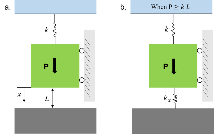Figure 4. Simplified physical problem representing how contact force is simulated in FEM software

The change in stiffness can be represented by the following,

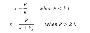
And the load versus displacement curve is reflected as follows in figure 5,

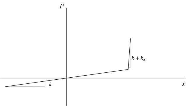Figure 5. Load displacement curve at contact closing when x > 0 and contact opening when x < 0. 

In midas FEA NX, is defined as the normal stiffness scaling factor. It should be defined with a reasonable size, since if is too small, large amount of nodal penetration would occur, and if is too large the analysis would experience convergence difficulty due to “bouncing”. The sudden change in stiffness at contacting surface as shown in figure 5 results in large nonlinearities in the finite element analysis, therefore, nonlinear solver is needed to model such behavior.

6. Examples of Contact Modeled in Finite Element Analysis 

Figure 6 shows the general contact modeled between two solid objects in Midas FEA NX. The user has defined the concave surface of the top object and the upper surface of the ground surface to be in contact. Therefore, when the concave surface of the top object is being pulled down and when the surfaces are within the algorithm searching distance, contact happens.

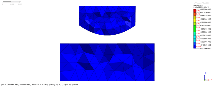
Figure 7 shows the lap joint under lateral tensile stress. To connect the two mesh sets whose nodes do not merge, welded connection is used. And figure 8 visualizes the structural connection through exaggerated displacement.

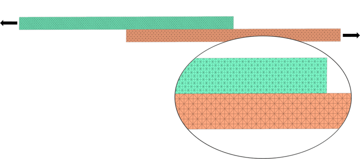
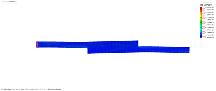
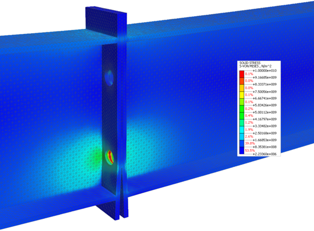
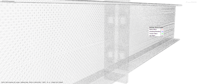
Figure 9 shows the von-mises solid stress at the splice I girder connection. Force and moment values at the separate ends of the I girders are initially obtained from general structural analysis result using 1D beam elements. In the solid model shown in figure 2, those loads are applied at the center node of the I beam ends. and rigid links are created between the center node and every node at the I beam ends. This ensures that the force and moments are applied uniformly at the beam end of the solid model. Bolt is simulated using a rigid element connecting the center of the bolt holes on each of the splice I girder connector plate. Bolting action is simulated by connecting the bolt rigid element with the hole surface nodes using rigid elements. General contact is established between the connector plates. Figure 10 shows the progressive plastic failure of the steel material around the bolting holes.

References

[1] R. Cook, D. Malkus, M. Plesha, R. Witt, Concepts and Applications of Finite Element Analysis, Fourth Edition, 2001, John Wiley & Sons Inc., New York, NY.

[2] Midas Information Technology, Analysis Reference Midas FEA NX, Chapter 5, 2021.