Moving Load Optimization in MIDAS CIVIL

1. Introduction

There are different types of loads to be applied on the bridge. Traffic loads are one of the leading actions in Bridges. The vehicle will move in both transverse and longitudinal directions. Therefore, moving load analysis is an important part of the bridge design. Moving load definition mainly consists of three steps

1. Defining the traffic lane
2. Vehicle Standard
3. Moving load Case

We can define a few traffic lanes manually, but we cannot judge that the lane position of the vehicle defined will create the maximum moment and force. This will lead to an approximate analysis. To perform an accurate analysis, we need to create multiple lanes along a transverse direction for a single load case. Defining multiple lanes manually is a time-consuming process. Along with that, we need to define multiple moving load cases. We can utilize the moving load optimization feature in MIDAS CIVIL.  This feature will help us to create the number of lanes required in the transverse direction by defining a single lane. Let us see the procedure for the moving load optimization in MIDAS CIVIL.

2. Moving load Optimization in MIDAS CIVIL

Moving load optimization allows you to find the number of loaded lanes and the exact position of vehicles in the transverse direction and a longitudinal direction, which will give the most critical responses.

Applicable Codes for Moving Load Optimization
AASHTO Standard
AASHTO LRFD
BS
CANADA
CHINA
EUROCODE
POLAND Standard
PENNDOT
RUSSIA
SOUTH AFRICA

The following parameters need to be defined for moving load optimization
      a. Optimization of lane and lane width
      b. Generate analysis lane
      c. Wheel spacing
      d. Margin
      e. Offset distance to the lane center

a. Optimization lane and lane width:

The optimization lane is equal to the carriage-way width for which the vehicle should be placed at a different location in the transverse direction. Lane width is the width of a single design lane.

b. Generate Analysis Lane:

There are two methods in MIDAS CIVIL to generate the m number of lanes for moving load optimization.
Where m = number of lanes generated in transverse direction using moving load optimization

Method 1:
Number of lanes to be generated for analysis =m =2^N +1
Example if N =1, then number of lanes generated = m =2¹ +1 = 3

Method 2:
Offset from centerline:
The vehicle will be placed at the centerline of the lane defined. Then it moves with the distance mentioned in the Offset from the centerline towards the left side and right side as shown in Figure 1.

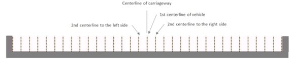
A vehicle centerline that does not satisfy the requirements of margin and minimum spacing between vehicles will be removed from the vehicle application.

c. Wheel Spacing:

It is the transverse spacing between the wheels in an axle. For influence line analysis, the program automatically applies a load equal to "Load ÷ no. of wheels" to each wheel.

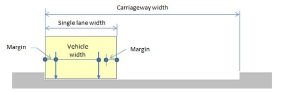
d. Margin:

It is the minimum distance between a wheel load and the boundary of a single lane. The centreline is denoted with a red dotted line and the boundary line with a blue dotted line. Margin should be so chosen that the sum of vehicle width and 2 times margin does not exceed the single-lane width. The margin distance is shown in Figure 2.

Example:
Single Lane width = 3m
Vehicle Width = 2m
The Sum of the Margins on each side should be less than (3-2=1m)

Distance between two vehicles for generating another lane is a maximum of
a. Two times the margin
b. Min Vehicle clear distance

Stradling lane type in moving load case is supported for BS and Eurocode such as HB load, Special Vehicles, and Load Model 3. The vehicle will straddle from one lane to another lane.

e. Offset distance to the lane center:

It is the distance from reference nodes to the center of the carriageway width.

3. Application in MIDAS CIVIL

To explain the output of the two methods, present in the generate analysis lane, I have taken one example for each method and shown the images of the lanes generated by the software automatically.

Example of Method 1:
The total width of the bridge is 9.65m. The width of each crash barrier is taken as 0.45m.
The clear Carriageway width is 9.65-2*(0.45) =8.75 m,
Number of lanes generated for N=1 is m= 2¹ +1 = 3.
The inputs for method 1 are shown in Figure 3.

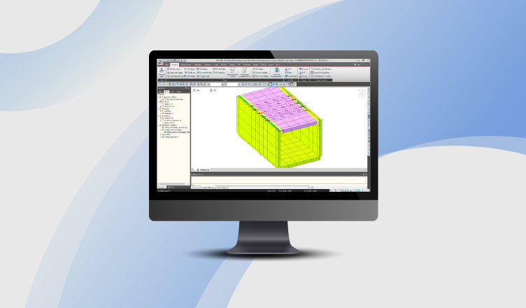
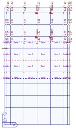
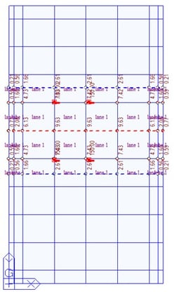
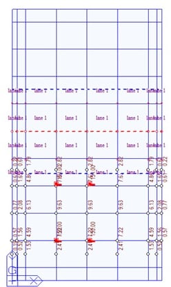
The lanes are automatically generated by the software as shown in Figures 4 to 6. The red dotted line represents the center line of the lane defined and the blue dots represent the boundary of the lane. Axle loads are represented by the red vertical line in the 3D view and the red dot in the top view.

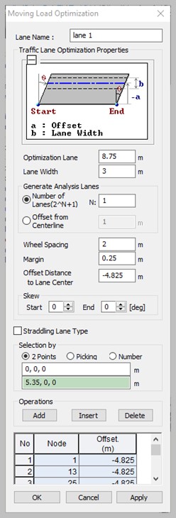
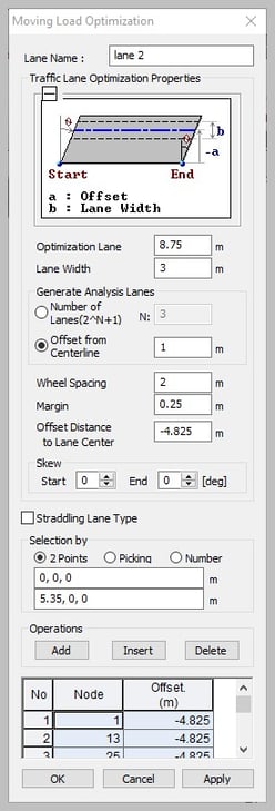
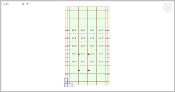
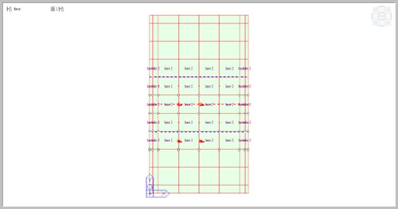
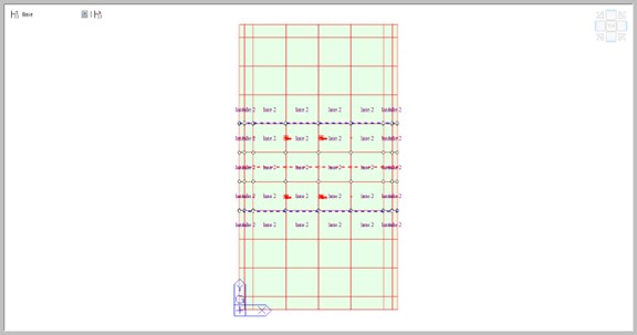
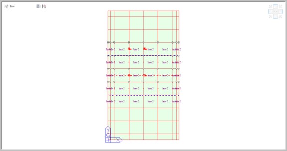
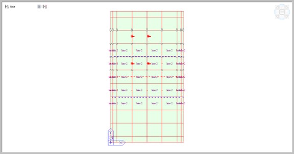
Example of Method 2:
The optimization lane width is taken as 8.75m and the single lane width as 3m. Offset distance from the center line is taken as 1 m. The traffic surface Lane is defined at the center of the carriage-way width at an offset distance of -4.825 m from the origin. Five lanes are automatically generated by the software with an offset distance of 1 m from the center line of the adjacent vehicle. It continues to create the lanes till the spacing for the end lane is not sufficient. The input data for method 2 in MIDAS CIVIL is shown in Figure 7.

The number of lanes generated in this method is m=5. The five lanes are automatically generated by the software as shown in Figures 8 to 12.

Figure 10: Lane 3 of method 2

 

 

Figure 11: Lane 4 of method 2

 

Figure 12: Lane 5 of method 2

 

4. Conclusion

Defining the ‘m’ number of lanes manually is a time-consuming process. The Moving load optimization feature in MIDAS CIVIL makes the job simple. It defines the ‘m’ number of lanes if we define a single lane manually. It generates the influence lines/surfaces for the ‘m’ number of lanes and gives precise results for moving loads in the transverse direction. This feature will become handy when you need to define lanes in large carriageway-width bridges with multiple load cases. The user can choose any one of the methods as per convenience.