 Get Started midas Civil
 Featured blog of this week

Interpretation of Dynamic Eigenvalue Analysis in Bridges
Please fill out the Download Section (Click here) below the Comment Section to download the Ebook
Table of Contents
1. Basic Concepts of Dynamic Analysis and Field of Application
2. Variables that affect the dynamic behavior
2.1 Mass
2.2 Stiffness
2.3 Structural damping
2.4 Model discretization
3. Types of modal analysis and interpretation of results
4. Atypical results in general modal analysis
5. References and further reading materials
1. Basic Concepts of Dynamic Analysis and Field of Application
Why do we need to understand the dynamic behavior of a structure? The answer to this question may be very extensive. From the structural point of view, it may be one of the following:
1. Structures must be designed to withstand earthquakes with a certain level of damage depending on design code criteria, which is a phenomenon of forced vibration when the ground movement is generated, and free vibration when the ground movement stops.
2. Depending on the level of importance, an explosion could be considered a design event, which from the dynamic point of view represents a strong or weak impulse that produces movements in the structure depending on its proximity to the source, in addition to the force generated by the pressure wave of the explosion itself. Bridges are quite susceptible to this, especially on major roads.
3. Several events could generate a direct impact force on the structure. In the case of bridges, it could be a collision of a vehicle traveling on the bridge or colliding with the substructure if it passes under it. Also, a ship can collide with the bridge when it crosses a navigable body of water.
Having explained the above, we can proceed to study the basic concepts and variables involved in dynamic behavior. The equation of motion for a one-degree of freedom structure is: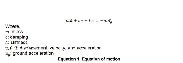
When an external excitation occurs (), the behavior of a structure depends on how the acceleration is distributed in the system mass, the effectiveness of the damping with which it is equipped, and the level of restriction that stiffness imposes against displacements.
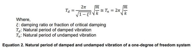
If we assume that there is a low damping, less than 15% (Duan et. al, 2000), as is normal in many structures such as bridges, then the problem is simplified, and we can assume that the damped dynamic behavior is very similar to that of undamped:
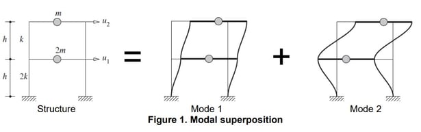
But we know that a real structure has multiple degrees of freedom, and by using the modal analysis method, its behavior can be assumed to be the superposition of the behavior of each independent vibration mode. Graphically:
The dynamic properties that can be obtained from an eigenvalue analysis include:
- Natural mode: A natural mode pertains to free vibration in an undamped system. 1st mode, 2nd mode and nth mode represent the order in which least energy is required to deform the structure.
- Natural Period: A natural period is the time that it takes to freely vibrate the structure into the corresponding natural mode one full cycle.
- Fundamental mode or period: The first natural mode or period of the structure. This is the vibration mode that requires the least energy to deform the structure as it was modeled.
- Main mode or period: Mode or period in ascendent order which effective mass is non-negligible. This concept is especially useful in numerical modeling, where not always the main mode or period matches the fundamental mode or period.
- Modal Participation Factor: The ratio of the influence of a specific mode to the total modes.
- Effective (modal) mass: Fraction of the total mass that it is activated in a vibration mode. The effective mass is determined from the modal participation factor.
Since each mode excites the structure in a different way, each mode can be associated with a particular vibration shape that contributes in a different way to the total behavior of the structure. The total effective mass is usually used as a control measure to know the minimum number of modes to include in the analysis, but other criteria are also used. The most common are:
- Include in the analysis a total number of modes at least three times the number of spans in the model. This criterion is the one adopted by AASHTO, which in its 2020th version is included in 4.7.4.3.3.
- Include in the analysis a total number of modes such that the total effective mass is at least 90% of the total mass of the structure. This is the traditional criteria in many design codes and applicable to conventional bridges.
- Include in the analysis a total number of modes such that the total effective mass is at least 95% of the total mass of the structure. This criterion applies to unconventional bridges or bridges with a large number of spans, where the participation of high modes can be very relevant and critical for certain components (FHWA, 2019).
As an example, consider the following bridge modeled in midas Civil:
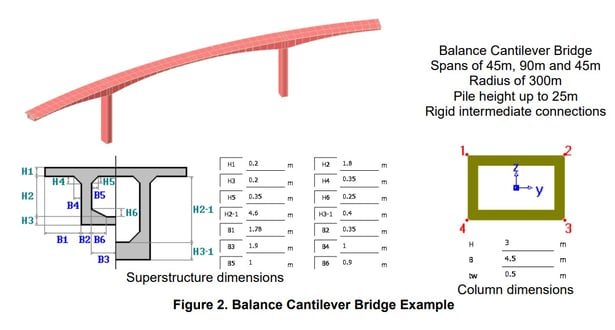
We can classify the balance cantilever bridge as conventional. To find the minimum number of modes that meets a 90% cumulative effective mass, we summarize the results of the first 3 main modes in the longitudinal direction:
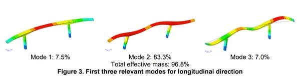
For the longitudinal direction, two modes would be sufficient to fulfill the 90% criteria, but according to AASHTO this bridge requires at least nine modes of vibration to be analized, even when we have 97% of the total mass covered in the accumulated effective mass. In most of the bridges, AASHTO’s criteria would be enough, but it is good to check the effective mass in all cases.
We have presented some of the main variables involved in the dynamic behavior of the structures as can be obtained from an eigenvalue analysis, both for SDOF and MDOF structures. Although we are going to study those variables in further detail in the next chapters, the general topic of the dynamic behavior of structures can be studied in detail in some textbooks like:
- Dynamics of structures – Anil K. Chopra (2020)
- Structural dynamics of earthquake engineering – Rajasekaran (2009)
- Bridge Design Handbook – Lian Duan, Murugesu Vinayagamoorthy, Rambabu Bavirisetty (2000)
2. Variables that Affect the Dynamic Behavior
In this chapter, we will study the variables that were introduced earlier from the numeric modeling perspective.
2.1 Mass
In Equation 2, we can observe that the vibration period is proportional to the mass. To the extent that a bridge has more mass that can vibrate, it will be subjected to larger forces that will have to be resisted by the structural members.
In numeric modeling, mass sources consist in masses that come from the modeled part of the structure (source 1) and masses that come from the part of the structure that was not modeled (source 2). For example, traffic barriers are not usually considered in the model, but they increase the mass of the structure, and they should be accounted for in dynamics.
In midas Civil, mass source 1 is considered when we convert self-weight into masses and mass source 2 is considered when (other) loads are converted to masses. Graphically:
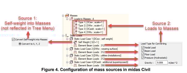
Unlike other programs, midas Civil easily prevents duplication of masses, even when Self-weight load case is used in both mass sources, source 1 is only going to take the part of the load that comes from the materials and section dimensions, and source 2 is only going to take the part of the load that is directly input as load (nodal, beam, floor, or pressure). It is also important to define if some portions of non-permanent loads are going to be converted as masses, which is common for long span bridges.
Other aspect that requires consideration is where torsional or high-skew behavior needs to be captured for some bridge superstructures. For example, consider a box girder bridge. A simple numeric model can be used for analysis and design if little or no torsional effects are expected, using only one line finite element with the cross section of the entire bridge deck assigned to it. This is called a spine model. This type of modeling cannot capture wide roadway effects, high-skew effects or torsional effects. For those effects, grillage models are very effective.
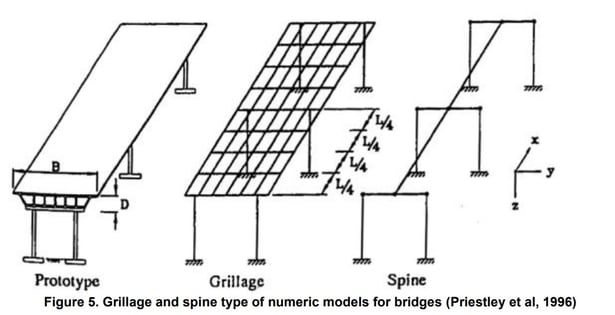
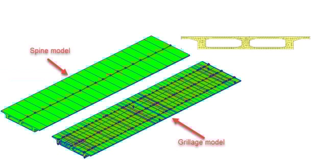
Now, regarding the dynamic behavior of bridges with high-skew or wide decks, spine models cannot reflect the eccentricity of the masses. In that case, eccentric masses rigidly connected would need to be considered in spine models, but this becomes impractical where software can automatically handle grillage models to better capture this and other effects in the bridge, along with the design. For example, in midas Civil, a spine and grillage model for the same two-cell box girder bridge is shown next, and the grillage model was developed using the Grillage model wizard:
In terms of numerical modeling of masses, it is important to consider the six components of the masses: three translational and three rotational masses. The rotational masses could be transformed into a pair of translational masses with equivalent distance in between.
There are two general ways to consider masses in models: distributed and lumped masses. Midas Civil uses lumped masses in analysis for efficiency.
2.2 Stiffness
From Equation 2, it is observed that the vibration period is inversely proportional to the stiffness. To the extent that the bridge is stiffer, the vibration period will be smaller. If the vibration period is small, it will probably remain in the plate of the design spectrum (higher seismic demands).
The stiffness of the elements used for static analyses are usually suitable for dynamic analyses, according to the hypotheses allowed in many design codes. However, there are numerous reasons why this is not theoretically correct.
It is generally accepted that the behavior of a bridge under operational loads is linear. In these cases, gross stiffness is used, but it is possible that, for events such as an earthquake, the level of cracking of the concrete elements is such that the stiffness is greatly reduced. However, many design codes allow gross stiffness to be used even in dynamic analysis.
According to the research of Priestley (2003), in the case of circular columns, depending on the level of axial load and the amount of reinforcement, the stiffness could be affected in different proportions:
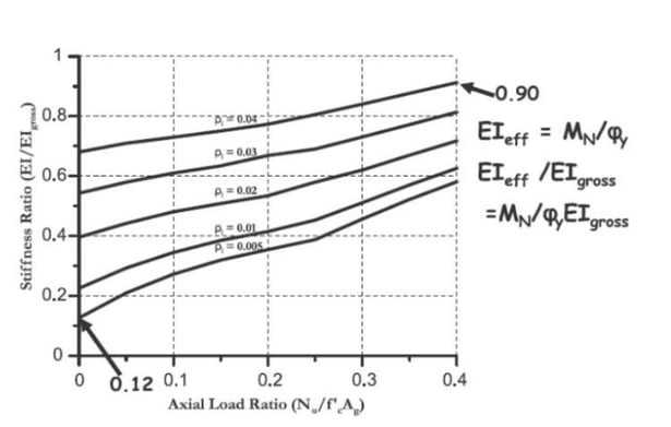
Using the previous values as an estimation for other cross section shapes, for the bridge of the Figure 2, the axial load caused by its own weight is 31500 kN, which translates into a stress of 4.85 MPa, 14% of the compressive strength of 35 MPa. Assuming the bridge is located in a high seismic zone, for an axial load ratio of 14%, the stiffness can vary between 40 and 75% of the gross flexural stiffness. Below, the results of the first three vibration modes are compared:
|
Vibration periods (s) |
Effective-to-gross flexural stiffness |
||
|
100% |
75% |
40% |
|
|
Mode 1 |
1.01 |
1.11 |
1.34 |
|
Mode 2 |
0.86 |
0.93 |
1.14 |
|
Mode 3 |
0.36 |
0.40 |
0.51 |
As can be seen, as the vertical elements of the bridge crack more, they will be more flexible and then in the seismic analysis they will benefit from a lower seismic demand.
The midas Civil program allows you to assign stiffness values by element, by section and by load case. In this way, different rigidities could be assigned for each bridge load scenario. In the previous example, the stiffness of the two columns was assigned by section.
2.3 Structural Damping
The damping is the process by which the vibration of the structure diminishes in amplitude. The more the damping in a structure, the less it will vibrate. There can be several damping sources in a structure: friction between materials, micro and macro cracking, hysteretic material behavior, yielding of ductile materials, hinging, slip in the connections, etc.
The real damping behavior is not frequency dependent as shown in the Equation 1, but amplitude dependent. However, it is very convenient to simplify the formulation of damping because it reduces in great manner the computational effort, and it has been demonstrated that the results are in good agreement. In structural analysis, the damping is usually represented by the damping ratio (as a fraction of the critical damping).
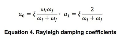
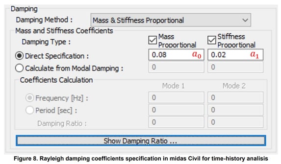
For eigenvalue analysis, the damping ratio is not needed as the damping becomes uncoupled if we consider that the dynamic properties are very similar to those undamped. However, when performing seismic analysis where we need to obtain structural responses, the damping properties are input directly for specific or all modes in response spectrum analysis, and a Rayleigh damping formulation (Equation 3) is often used for time-history analisis, where and are the coefficients for mass and stiffness proportional damping, respectively:

From dynamics, it can be demonstrated that:
Most design codes specify a 5% damping ratio for concrete structures. If we use Rayleigh damping for some typical period values (0.25 to 1 seconds – 4 to 1 Hz), the damping rations follow the curve:
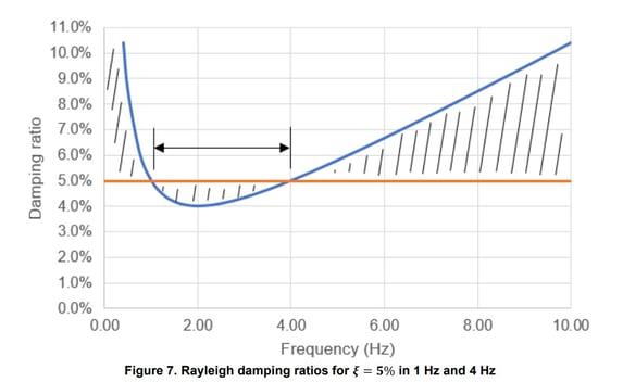
And if we consider that this is a good estimation of damping, we will find that there is no constant damping in the range of interest (or any other zone!) even when we try to reproduce a more constant curve.
There are two scenarios where one would need to pay close attention to the damping: where response spectrums don’t match the structure damping ratio, and where time-history analysis needs to be configured (often) using two frequencies as reference for the representation of the entire damping behavior of the structure. Neither of the two scenarios are studied in this article but are presented because of the close relation to the eigenvalue analysis problem.
2.4 Model Discretization
Although we know that the reality is that matter is continuously distributed in the volume of the members, numerical modeling concentrates the masses in the nodes. Below are three models of a simple span bridge:
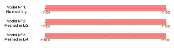
Midas Civil as a finite element program, considers only those masses that can move. In the models, two translational degrees of freedom have been considered for each model node: vertical and horizontal. Then, each tributary mass to the free nodes could translate in two ways.
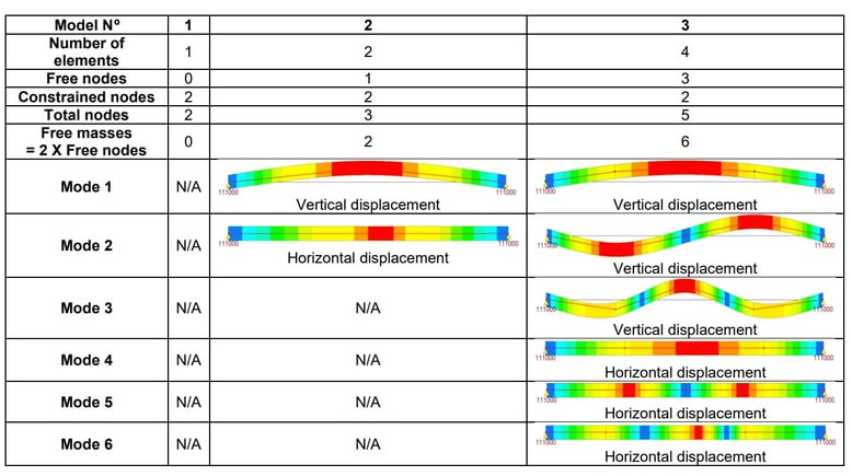
As you can see, the first model does not even produce vibration mode results. In fact, the program warns when running the analysis: ERRORS ENCOUNTERED. MIDAS JOB TERMINATED. REFER TO .OUT FILE. Yet, this model is valid for performing static load analysis, but it would be unsuitable for dynamic analysis due to poor discretization.
3. Types of Modal Analysis and Interpretation of Results
Eigenvalue analysis provides dynamic properties of a structure by solving the characteristic equation composed of mass and stiffness:

As stated in chapter 1, eigenvalue analysis does not consider the masses that are constrained. Therefore, effective modal mass relates to the total mass that is not constrained and not the total modeled mass.
There are several types of eigenvalue analysis numerical integration methods. Three of them are very effective for numerical modeling:
- Subspace iteration method.
- Lanczos method.
- Ritz vectors method.
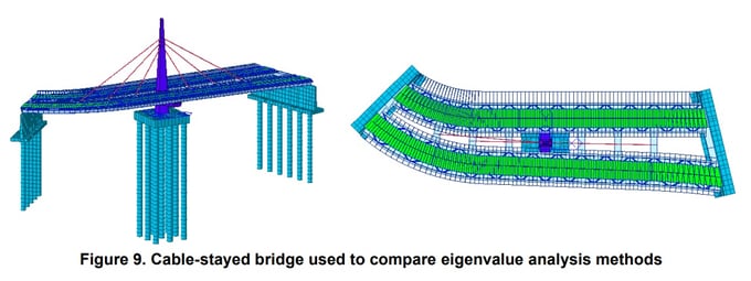
To compare the methods, a cable-stayed bridge numeric model is used. The main characteristics of the bridge are summarized:
- Semi-fan cable-stayed bridge.
- Steel box girder superstructure.
- 4 lanes total. 2 lanes per box girder.
- 2 meters total span
3.1 Subspace Iteration Method
This method was developed by professor E. L. Wilson. Pace iteration matrix calculation is used to perform eigenvalue analysis. This method is effectively used when performing eigenvalue analysis for a finite element system of a large scale (large matrix system) in which higher modes influence is not very high. This method is commonly used among structural engineers.
Using the example model, the main results are:
- Longitudinal (X) vibration period: 1.38576 s
- Longitudinal (X) accumulated effective mass: 72.50%
- Transverse (Y) vibration period: 1.75131 s
- Transverse (Y) accumulated effective mass: 72.26%
- Number of analyzed modes: 55
Other results are:
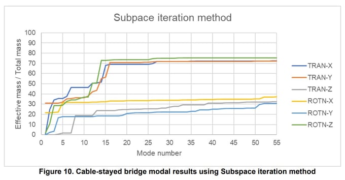
Further conclusions are summarized:
- The bridge shows more flexibility in the transverse direction than in the longitudinal direction.
- The number of analyzed modes was not able to capture the total mass or even the 90% of the total mass of the structure.
- Translational behavior of the model was better captured than rotational.
- There is little influence of modes 15 to 55 to the overall dynamic behavior of the bridge.
- Torsional or rotational behavior may not be fully captured.
- The model shows important influence of higher modes.
3.2 Lanczos method
Tridiagonal matrix is used to perform eigenvalue analysis. This method is effectively used when performing eigenvalue analysis for lower modes.
Using the example model, the main results are:
- Longitudinal (X) vibration period: 1.36886 s
- Longitudinal (X) accumulated effective mass: 72.32%
- Transverse (Y) vibration period: 1.72976 s
- Transverse (Y) accumulated effective mass: 72.07%
- Number of analyzed modes: 55
Other results are:
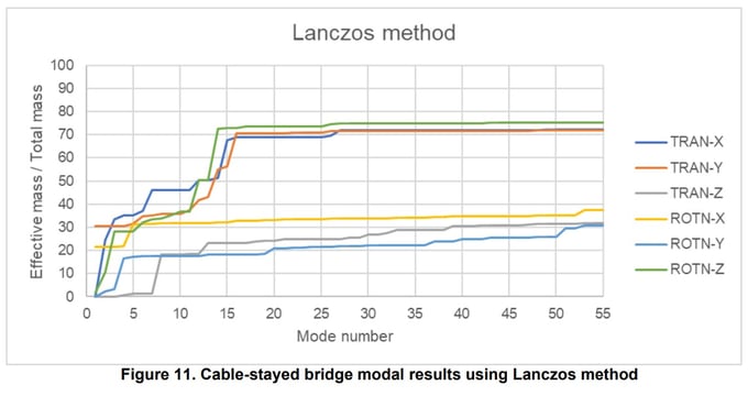
In this case, similar results to the subspace iteration method were obtained, therefore the same conclusions could be established.
3.3 Ritz vectors method
Unlike the natural eigenvalue modes, load dependent Ritz vectors produce more reliable results in dynamic analyses with relatively fewer modes. This method is an extension of the Rayleigh-Ritz approach, which finds a natural frequency by assuming a mode shape of a multi-degree of freedom structure and converting it into a single degree of freedom system.
The Ritz vectors are generated reflecting the spatial distribution or the characteristics of the dynamic loading. Therefore, this method requires a load that can be used as directional vector for the modes to be found. In the extent that the input vectors are close to a real modal vector, the eigenvalue will be close to the eigenvalue associated with the vibration mode. The modeling program will automatically adjust the initial vectors so that they match the mode shape vectors.
The Ritz method finds the modes with higher effective mass, which makes it more effective with fewer entered number of modes than the previous methods.
Midas Civil can use static load cases, uniform ground acceleration and general link forces as initial vectors. The easiest way to input initial vectors is to use ground acceleration in the direction of interest.
Using the example model, the main results are:
- Longitudinal (X) vibration period: 1.36886 s
- Longitudinal (X) accumulated effective mass: 99.97%
- Transverse (Y) vibration period: 1.72976 s
- Transverse (Y) accumulated effective mass: 99.99%
- Number of analyzed modes: 55
Other results are:
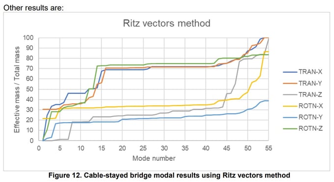
Further conclusions are summarized:
- The bridge shows more flexibility in the transverse direction than in the longitudinal direction.
- Lower modes results are more identical to Lanczos method. This may point to the accuracy of Ritz vectors method to all type of modes.
- The number of analyzed modes was able to capture almost 100% (or at least close to 90% in some cases) of the total mass of the model in every direction. For the rotational Y direction, lower precision was obtained as long as the accumulated effective mass was about 40% of the total mass.
- Translational and rotational behavior of the model was well captured.
- There is little influence of modes 15 to 42 to the overall dynamic behavior of the bridge. The number of the modes only indicates the order in which they were obtained, so we can establish that modes 43 to 55 in this case are different than those found in previous methods and were more important to the overall behavior of the bridge.
- Torsional or rotational behavior may be well captured but can be improved.
- The model shows important influence of higher modes.
3.4 Comparison of methods
To summarize the characteristics of the eigenvalue analysis methods, you can refer to the following table:
Table 1. Comparison of eigenvalue analysis methods
|
Method |
Subspace iteration |
Lanczos |
Ritz vectors |
|
Requires number of modes to be found |
Yes |
Yes |
Yes |
|
Requires initial load vector |
No |
No |
Yes |
|
Order of eigenvalues found |
Least energy to deform the structure |
Least energy to deform the structure |
Least energy to deform the structure and higher effective modal mass |
|
More effective in |
Large scale models |
Small scale models |
Large scale models |
|
Additional use |
Detection of errors in numerical modeling |
Detection of errors in numerical modeling |
N/A |
|
Frequency of use |
High |
Small |
Medium |
4. Atypical Results in General Modal Analysis
In some cases, particular results in modal analysis can challenge the engineer’s criteria to judge the reliability of the results. The following cases are set in bridge scenarios:
- Case #1: Many numbers of modes are required to reach ~100% of effective mass.
For structures whose model requires great number of degrees of freedom or where the model is composed of members with very different stiffness, many numbers of modes are required to reach an effective mass close to 100% of the total (free) mass of the model. Let’s consider the Gongchon bridge, a cable stayed bridge with the dimensions shown in the following figure:
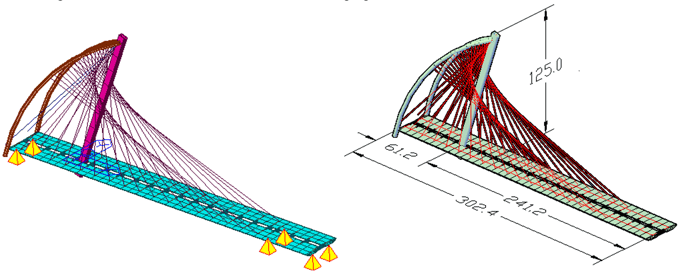
This model has 234 nodes and 273 finite elements (36 tension only elements -cables- and 237 beam elements -deck and pylons-). The number of degrees of freedom is not what’s very high in this case but the variability in the stiffness that the cables provide to the bridge overall dynamic behavior. Using the default method of eigenvalue analysis of midas Civil, the Lanczos method, this bridge requires about 500 modes to reach ~100% of effective mass. The results are reflected in the following figure:
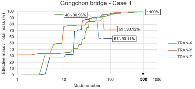
Figure 16. Effective masses for the Gonchong bridge eigenvalue analysis
The graph shows in a convenient logarithmic layout the results of the first modes in a detailed form and the higher modes with a reduced detail, considering the higher variability for the left part of the curves. The 90% of effective mass is reached in 51, 69 and 40 modes for the translational X, y and Z directions, respectively. This is a strong contrast when compared to the 500 modes required for the ~100%.
In this case, the fact that the bridge has so many elements with mass that are flexible is the main reason of the great number of required modes to reach ~100%. This will impose certain computational cost to the modal analysis but is not necessarily a reason to doubt about the reliability of the results or the model itself. However, if there is a way to simplify the model without loosing the desired level of detail, it should be considered for a next phase of the modeling process.
- Case #2: >90% effective mass is not reached even when the number of modes is increased.
In structures with similar or more pronounced characteristics than those considered in the Case #1, i.e., structures whose model requires great number of degrees of freedom or where the model is composed of members with very different stiffness, it may be difficult to even reach 90% of the effective mass in the eigenvalue analysis.
Considering the same Gonchong bridge of the Case #1, for the untrained eye, the starting point to set a number of modes would be 3 X 2 (number of spans) = 6, which would be AASHTO’s criteria (notice that AASHTO code is not applicable to this type of bridges). But when it is proven that this is very low to reach 90 or ~100% of effective mass, the number of modes will increase blindly. After a couple of trials and errors, and the number of modes has just passed 100, 200, 300, 400, it may be worrying to see this atypical situation.
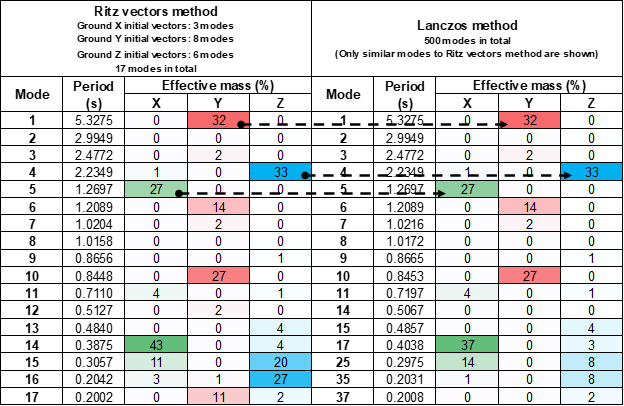
As we have already stated, this does not mean that there is an error in the model, but it would be very convenient to use a method like Ritz vectors to reduce the number of required modes. This will reduce the computational cost at a good level in most cases. For the Gonchong bridge, the required number of modes using Ritz vectors method is 17 in total to reach at least 90% of effective mass. In the following table, the analogous modes from the Laczos method that was used for the Case #1 are shown, and the good correspondence of the results is proven (mostly for the X and Y direction):
- Case #3: The fundamental modes are not the main modes.
When we perform an eigenvalue analysis for a 3D model of a bridge, it is expected that there will be a strong differentiation between the longitudinal, transverse, and vertical modes of vibration if the bridge is regular or there is little influence of irregularities. Also, we expect that the fundamental modes are the main modes for each direction, but this is not always the case.
Using the same example of the Gongchon bridge, notice that the first mode with no null effective mass in X direction is 4 with 1%. Because of the definition of this concept, this would be the fundamental mode for the X direction, but it certainly does not capture any significant dynamic behavior in this direction. Furthermore, the mode 5 has an effective mass of 27%, but it is the mode 14 which possesses the higher effective mass of 43%. It would be appropriate to call the mode 14 as the main mode for the X direction as this is the mode that better explains the overall bridge behavior for this direction.
Main modes are helpful to understand and simplify the behavior of the bridge. Some design methods are based on a specific mode (usually the fundamental mode), but when the bridge structure behaves in an atypical manner, good engineering criteria should be used to properly select the dynamic parameters of the structure to feed those design methods.
5. References and further reading materials
- Bridge Engineering HandBook - Wai-Fah Chen (1999)
- Manual for Refined (Modeling) Analysis in Bridge Design and Evaluation – FHWA (2019)
- Eurocode 8 - Design of structures for earthquake resistance - Part 2: Bridges (EN 1998-2: 2005)
- Response Spectrum Analysis in midas Civil - Pratap Jadhav https://www.midasbridge.com/en/blog/project_tutorial/response-spectrum-analysis
- Dynamic Analysis of Fan, Semi-Fan and Harp Type of Cable-Stayed Bridges - Rohan Agarwal https://www.midasbridge.com/en/blog/bridgeinsight/dynamic-analysis-of-fan-semi-fan-and-harp-type-of-cable-stayed-bridges
- Dynamic Analysis of Footbridges as per Eurocode - Jan Blazek https://www.midasbridge.com/en/blog/casestudy/dynamic-analysis-of-footbridges-as-per-eurocode
- Elastomeric Bearings for Bridges: Stiffness and Tips for Modeling – Cristian Londoño https://www.midasbridge.com/en/blog/bridge-insight/elastomeric-bearings-for-bridges-stiffness-and-tips-for-modeling
- https://www.midasbridge.com/en/solutions/dynamic-analysis


.png)