[Part 1. Modal method] Initial Load Optimization in Nonlinear Time History Analysis

📢 To check the entire series, click here

• [Part 1. Modal method] Easy Guide to Considering Initial Load in Boundary Nonlinear Time History Analysis

• [Part 2. Direct Integration method] Easy Guide to Considering Initial Load in Boundary Nonlinear Time History Analysis

• [Part 3. Damping method] Easy Guide to Considering Initial Load in Boundary Nonlinear Time History Analysis

In MIDAS CIVIL, elements with nonlinear properties such as seismic isolation, vibration control bearings, and dampers can be represented in the analysis model with the General Link option.

Example with General Link (by MIDAS Tutorial)

   Unlike analysis models that use elastomeric bearings and pot bearings, which have linear behavior, an analysis model using a General Link that simulates bearings with nonlinear behavior performs a Time history analysis.

   There are many factors to consider in boundary nonlinear time history analysis. In this content, we will talk about how to consider initial loads among those factors.

A. The reason why we need to consider initial loads

   In nonlinear time history analysis, the presence of initial load can significantly affect the results depending on what kinds of general links are used.

   In particular, for Friction Pendulum bearings (FPBs), damping due to friction should be considered about axial load. Simply, the frictional force is the product of friction coefficient and normal force, so the behavior can differ greatly depending on the axial load.

   If the self-weight of the superstructure is not considered as an initial load, the frictional force decreases and accordingly, there can be abnormal displacement under lateral loads.

   Therefore, it is necessary to conduct a time history analysis considering the vertical load (dead load), i.e. initial load.

- Defines time history of seismic wave (Load > Dynamic Load > Time History Functions),
- Defines time history load cases,
- Converts the time history into Ground Acceleration based on time.

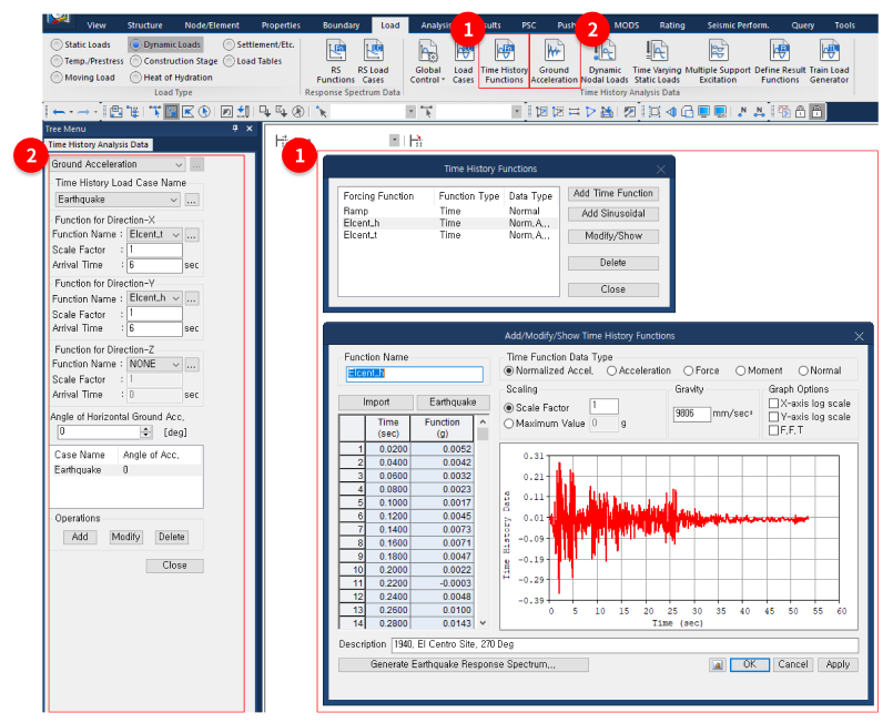Time History Functions & Ground Acceleration

   The method of applying seismic waves to the analysis model and combining the results with static analysis results does not apply to analysis models that use nonlinear boundary conditions.

   When performing Response Spectrum Analysis (RS Analysis) for elastic support, the principle of linear superposition is applied for each load since it is a linear static analysis.

   Therefore, static load cases and seismic load cases can be combined in load combinations according to the design code.

   However, in the case of nonlinear boundary conditions, the linear superposition of each load is not applicable, and the initial load (dead load) needs to be considered.

B. How to apply initial loads in MIDAS CIVIL

1. Option to apply initial loads

   Let's see how to apply the initial loads.
   Initial loads can be applied through Order in Sequential Loading, or Initial Load (Global Control) in Time History Load Case.

- In the Modal method, Order in Sequential Loading is activated.
- In the Direct integration method, you can select between Order in Sequential Loading and Initial Load (Global Control).

Order in Sequential Loading and Initial Load (Global Control)

   In this content, we will discuss the method of considering initial load and its precautions when selecting the Nonlinear Modal method. There are two ways to consider the initial load: one is to consider the Static Load Case as the initial load, and the other is to convert the Static Load Case into a Time History Load Case and then consider it as the initial load.

   In this content, we will compare the results of these two cases to determine which method should be used to apply the initial load.

   The target model is a bridge model represented in Lead Rubber Bearings (LRBs).

Lead Rubber Bearings (LRBs)

2. Load Cases that can be applied as initial loads

   In the Nonlinear Modal method, the initial loads are considered through "Order in Sequential Loading".

   The load cases that can be considered as initial loads are as follows:

1) ST(Linear Static Load): Static load case

2) TH(Time History Load): Time History Load Case which is converted from Static Load Case using Ramp Function (Time History Load Case definition is required when applying converted TH load)

   There are two cases: ST (Dead) load input as self-weight and TH (Dead) load converted from ST (Dead) load using the Ramp Function.

   Which one is the appropriate method?
   The answer is simple.

   If you select Static load case as the initial load for time history analysis, you will receive the following [Warning] message.


[Warning] message

   Here, the Force Type General Link refers to an element that can define non-linear properties as shown in the below figure.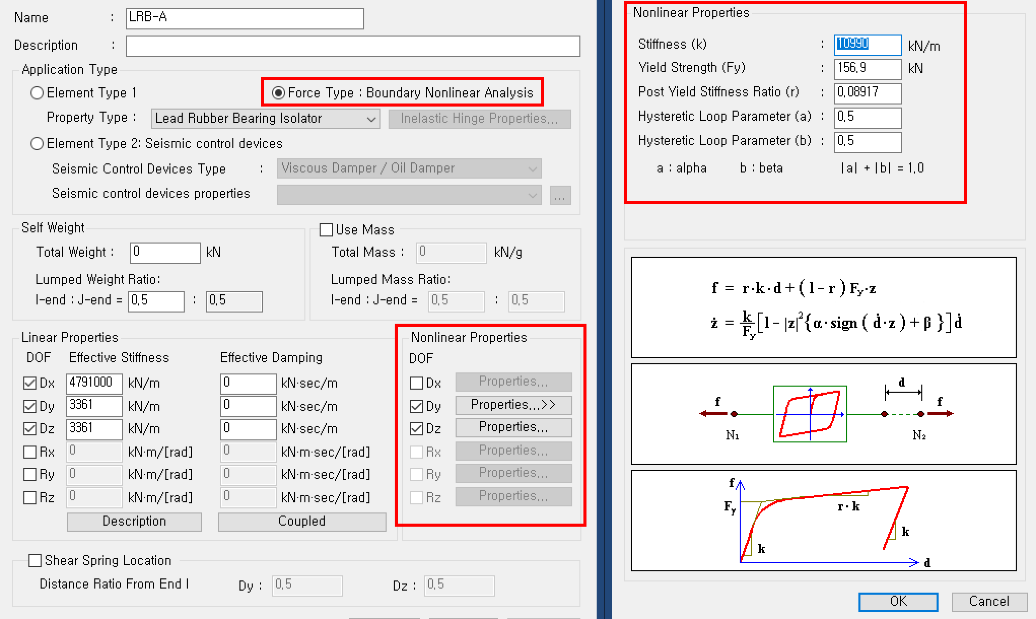

Force Type General Link

   When the initial load is set to ST (Dead load),
- It can be seen from the Result Table that the static analysis results are simply added to the results of the time history analysis. In other words, it means simply adding the results together, without performing any additional analysis related to time history analysis.
- ST(Dead load) cannot be applied as an initial condition in the time history analysis. Therefore, time history analysis proceeds without considering the initial load.
- The same words are written in the [Warning] message.

   The reason why the result of ST load cannot be selected as the initial load in time history analysis is as follows:
- If the member force from the initial static analysis exceeds the yield strength of non-linear boundary conditions (in the inelastic region), it cannot handle the exceeded internal force.

   Therefore, the answer to the previous question on the appropriate method to consider dead load as an initial load is,
   → It is appropriate to use TH (time history load case) as the initial load for models with nonlinear boundary conditions (such as General Link's damper, and Link with non-linear properties).

3. Example of setting the ST (Static analysis result) as the initial load

   Let's check the results of a bridge model that applies LRBs, and the load case for time history analysis is set as follows:

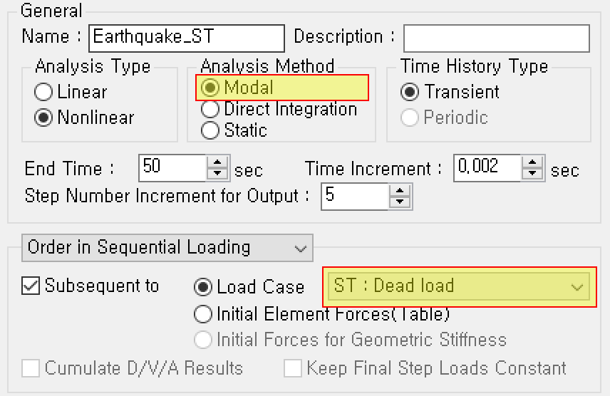Load case for time history analysis

   The analysis was performed by setting the Dead load as the initial load for the Static load case.

   After the analysis,
- Results Tab > Results Tables > General Link
- Check the ST (Dead Load) result and the Earthquake_ST (TH) result at General Link #4


Results of Dead load(ST) and Earthquake_ST(TH) at General Link #4

   The Min/Max output values at General Link #4 are shown in the Smart Graph.

Smart Graph results for the case where the initial load condition is set as ST (static analysis results)

   If the initial load is set as ST, the static analysis results cannot be taken, so it can be confirmed that member forces do not exist at 0 seconds.

※ To make the results more accurate, the Step Number Increment for Output must be set as 1.
For example, if you set this value as 5, the graph will output the results in every 5 steps, so the Max/Min member force may slightly differ.

   The graph shows the member force as follows:
- Max. axial force: 217.434 kN
- Min. axial force: -187.511 kN

   Note that the Min/Max axial force shown in the Result table and the Smart Graph are different.

   This is because non-linear boundary elements cannot take the static analysis results as initial conditions.**
   **In the conclusion, the Result Table shows the sum of (the time history analysis results starting from a zero initial load) and (the static analysis results for the initial load).

   Therefore, the values from the Result Table are calculated as follows:
   At the 60th Node (ith of General Link 4)
- The value of Earthquake_ST(max): -884.696 kN is calculated as,
- The value of Earthquake_ST(min): -1289.614 kN is calculated as,

   From the above, we can conclude:
- If ST load is considered as an initial load for time history analysis in a model with nonlinear boundary conditions, the results of static analysis are not applied as initial load conditions.
- As a result, the Min/Max values may differ between the Smart Graph and the Result Table.

   In conclusion, it is not appropriate to use ST load as the initial load for models with nonlinear boundary conditions to simulate the actual nonlinear behavior.

   Then, let’s talk about how to consider static load as the initial load.

C. Example of applying initial loads in Modal Superposition method

1. Time History Load Case for considering dead load as TH load

   In a Nonlinear Modal method for time history analysis of seismic waves, Ramp load is used as the initial load. (Time Varying Static Loads function)

   Let's check it in more detail.

   Loads > Dynamic Loads > Load Cases

   To apply dead load as an initial condition in time history analysis,
- After performing a time history analysis on dead load,
- Applying the corresponding member force as the initial load of the analysis

   Therefore, a specific Time History Load Case is required to convert the dead load (ST) into the time history load (TH).

   To apply the Nonlinear Modal method to the time history analysis of seismic waves, we also set the Analysis Type to "Nonlinear" and the Analysis Method to "Modal" for the dead load.

Time History Load Case (Dead load)

In the above figure,

i. End Time: Total analysis time for time history analysis

ii. Time Increment: How to set for time step within the total analysis time
(For example, in the above figure, since the total time is 5 sec and the time increment is 0.001 sec, time history analysis has 5000 steps.)

iii. Step Number Increment for Output: How often extract results from the total analysis steps
(For example, if you want every single of 5000 steps, you can type Time increment to 1. Or if you want the output in every five steps, you can type 5 then you can have the output of 1000 steps.)

iv. The Damping Method is set to Modal.
When the Analysis method is “Modal”, it is recommended to set Damping Method as "Modal".
When the Analysis Method is "Direct integration," it is recommended to set the Damping Method as "Mass & Stiffness Proportional". Otherwise, there may be a significant delay in analysis time.

v. Damping Ratio for All Modes: A value 0.999, which is close to 1, entered.
When dead load is applied, free vibration (damping ratio of 0) does not occur, so the analysis is carried out with a value close to 1.

3. Time-Varying Static Loads for Defining Dynamic Loads

4. Time History Analysis Considering Initial Load

D. Conclusion